Chapter 1: Interpretable ML Introduction

This chapter introduces the basic concepts of Interpretable Machine Learning. We focus on supervised learning, explain the different types of explanations, repeat the topics correlation and interaction.

§1.01: Introduction, Motivation, and History

ML has a huge potential to aid decision making process due to its predictive performance. However many ML methods are black-boxes and are too complex to be understood by humans. When deploying these models, especially in business critical or sensitive use-cases, the lack of explanations hurts trust and creates barriers.
We mostly think of using these methods to create the best predictor i.e. “learn to predict”, the other important paradigm is to understand the underlying relationships themselves i.e. “learn to understand” which is often the case in medical applications for example.
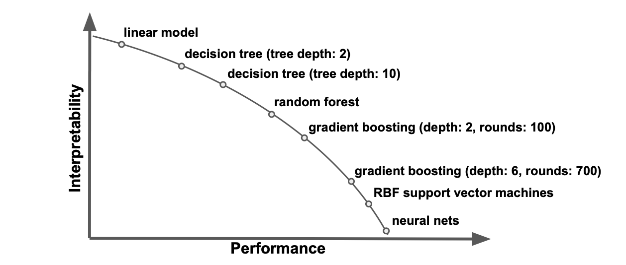
This is a fairly strong simplification of the performance-interpretability tradeoff as even a linear model can be difficult to interpret in the high dimensional space whereas neural-networks could be made very shallow.

We should always start with the simpler, less complex and more explainable model and only choose a more complex network if it is really needed. “Need” doesn’t always mean need for a better predictive performance.
GDPR, EU AI Act, and other regulations around the world makes explainable and interpretable ML even more important.

§1.02: Interpretation Goals

Interpreting models can serve a variety of important goals, including:

Uncovering Global Insights: This involves understanding the model as a whole across the complete input space, which can provide valuable insights into the dataset, underlying distributions, and relationships.
Debugging and Auditing Models: Gaining insights that help identify flaws, whether they are in the data or the model itself, is crucial for improving model performance and reliability.
Understanding and Controlling Individual Predictions: Explaining individual decisions made by the model can help prevent unwanted actions and ensure that the model’s predictions are used appropriately.
Ensuring Fairness and Justification: Investigating whether and why biased, unexpected, or discriminatory predictions were made is essential for ensuring that the model operates fairly and justly.

§1.03: Dimensions of Interpretability

Some models like shallow decision trees, simple linear regressions, are inherently interpretable and don’t require any specific methods post estimation. However they too can get become difficult to interpret if the trees are deep or if the regresion has too many interaction terms/engineered features.
For black-box models, we can develop techniques that are specific to one model (class), for e.g. summing up the Gini values across the tree.
We can also develop techniques/huerisitics that are model agnostic and universally applicable. This allows us to fit a predictor across many different model classes and then use model-agnostic technique.
There are different types of explanations:
1. Feature Attribution: produces explanations on a per-feature e.g. feature effects (ICE Curves, partial dependence plots, pendants in LR, saliency maps, SHAP, LIME) or feature importance (t-statistic, p-value). We can do this by varying the feature levels and inspecting the change in model prediction/variance/error/etc.
2. Data Attribution: identifies training instances most responsible for a decision (e.g. influence functions) i.e. which data points cause a certain model predicition?
3. Counterfactual Explanations: also known as contrastive explanations indentifies smallest necessary change in feature values so that a desired outcome is predicted.
Global interpretation methods explain the model behaviour for the entire input space by considering all available observations (e.g. Permutation Feature Importance, Partial Dependence plots, Accumulated Local Effects).
Local interpretation methods explain the model behaviour for single instances e.g. (Individual Conditional Expectation curves, LIME, Shapley Values, SHAP)
Within IML, there are multiple levels of interpretability analysis:
1. How to explain a given model fitted on a dataset? the object of the analysis is simply the fitted model $f_\theta$ like LR, NN, SVM, etc
2. How does an optimizer choose a model given the dataset? Here we look at the model selection process for e.g. decisions made by AutoML/HPO systems.
3. How do data properties relate to performance of a learner and its hyperparameters? Imagine if we had $n$ datasets and $m$ models. Here we try to understand the properties of ML algorithms in general i.e. if the dataset is large/small, low/high dimensional, sparse/dense then which algorithm performs better ?

§1.04: Correlation and Dependencies

Pearsons Correlation Coefficient:

\[\rho (X_1, X_2) = \frac{\sum_{i=1}^{n} (x_1^{(i)} - \bar{x_1})(x_2^{(i)} - \bar{x_2})}{\sqrt{\sum_{i=1}^n (x_1^{(i)} - \bar{x_1})^2} \sqrt{\sum_{i=1}^n (x_2^{(i)} - \bar{x_2})^2}} \in [-1, 1]\]

Geometric Interpretation: Consider just the numerator which is simply a sum of the product of $x_1 - \bar{x_1}$ and $x_2 - \bar{x_2}$. A multiplication of two numbers is simply the area under the rectangle represented by those points. The areas (numerator) determine the sign and the denominator simply scales it.

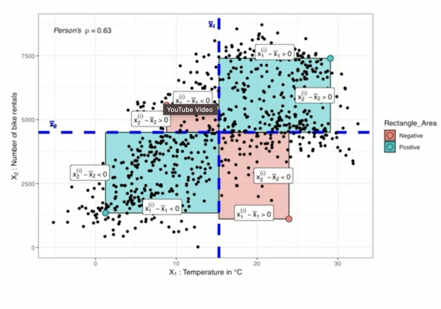
So if positive areas dominate then the correlation coefficient will be positive, if negative areas dominate then it will be negative. If the areas are equal then $\rho = 0$ which implies uncorrelated features.

Analytical Interpretation: Simply put if the direction/sign of the difference between an instance of the variable and the mean is the same i.e. if both $x_1$ and $x_2$ are smaller than their means OR both are larger than their respective means $\rightarrow$ positive correlation. On the other hand if the direction/sign is not the same $\rightarrow$ negative correlation.
An important thing to remember is that $\rho$ is a measure of linear correlation. For non-linear features, the correlation coefficient could be meaningless (more on that in a bit).

Coefficient of determination $R^2$:

Fitting a linear model and analysing the slope alone is problematic as for the same underlying data we could get different slopes. For example if we scale m to cm, then the linear regression’s slope will now be 100x for the same variable. Or if we negate a variable then the new coefficient would be negative.
$R^2 = 1 - \frac{SSE_{LM}}{SSE_{const}} \in [0,1]$ where $SSE_{const}$ is a constant model. $R^2$ is another measure to evaluate linear dependency which is invariant to scaling and simple transformation (depends on the transformation of course, if you multiply with another feature that is no longer a simple transformation) of the underlying data.
If $\frac{SSE_{LM}}{SSE_{const}}$ is 1, it implies that the fitted model is no different from a constant model implying no linear relation.

Dependence:

Definition: $X_j, X_k$ independent $\leftrightarrow$ the joint distribution is the product of the marginals i.e.
\[P(X_j, X_k) = P(X_j) \cdot P(X_k)\]
An equivalent definition (that can be derived using the above definition) is:
\[P(X_j \mid X_k) = P(X_j)\]
and vice versa implying that knowledge of the other variable has no effect on the conditional probability.
Measuring complex dependencies is difficult but but different measures exist:
1. Spearman Correlation measures monotonic dependencies via ranks
2. Information Theory approaches like the Mutual Information
3. Kernel based measures like Hilbert-Schmidt Independence Criterion (HSIC)
One very important thing to note is that independence implies $\rho = 0$, however $ \rho = 0 $ does not imply independence. A very simple example to illustrate this is to imagine $x_1, x_2$ such that $ x_1^2 + x_2^2 = 1$ i.e. they lie on the unit circle. From a linear perspective, there is no relationship and therefore the correlation coefficient will be close to if not 0. However there is an underlying quadratic relationship between the two variables.

Mutual Information

Mutual information describes the amount of information shared by two R.Vs by measuring how “different” the joint distribution is from the product of marginals. It is 0 if and only if the variables are independent.
\[MI(X_1, X_2) = E_{p(X_1, X_2)}[\log \frac{p(X_1, X_2)}{p(X_1) p(X_2)}]\]
Whereas Pearson’s correlation is limited to numeric (and linearly related) features, Mutual Information can be calculated for any kind of variables — discrete or continuous, numeric or categorical — as long as a valid joint probability distribution is defined.

§1.05: Interaction

Whereas feature dependencies concern only the data distribution, feature interactions may occur in structure of both the model or the data generating process. Feature dependencies may lead to feature interactions in a model.
Interactions: A feature’s effect on the prediction depends on other features e.g. $\hat{f}(x) = x_1 x_2 \Rightarrow$ Effect of $x_1$ on $\hat{f}$ depends on $x_2$ and vice versa. A function $f(x)$ contains an interaction between $x_j$ and $x_k$ if a difference in $f(x)$-values due to changes in $x_j$ will also depend on $x_k$ i.e.
\[E[\frac{\partial^2 f(x)}{\partial x_j \partial x_k}]^2 > 0\]
The mixed partial derivative measures how the rate of change of $f$ wrt $x_j$ changes when $x_k$ varies. Again, it measures how the rate of change varies. If this derivative non-zero, it indicates an interaction effect and the squared expectation ensures that we capture the overall magnitude of this interaction effect across the feature space.
If $x_j$ and $x_k$ do not interact, $f(x)$ is a sum of 2 functions each independent of $x_j, x_k$ i.e.
\[f(x) = f_{-j}(x_1,.., x_{j-1}, x_{j+1},...) + f_{-k}(x_1,...,x_{k-1},x_{k+1},...)\]
When features interact, we cannot interpret their effects on function output independently because:
1. The effect of changing $x_j$ depends on specific value of $x_k$
2. The function cannot be separated into additive components
3. The combined effect of $x_j$ and $x_k$ is different from the sum of their individual effects.
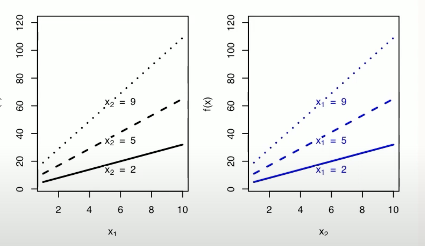
Visualizing Interactions: For a function with no interaction, the effect curves at different slices of a nother variable would be parallel whereas for functions with interactions, the effect curves would have different slopes or shapes.


When there is an interaction, the effect of one variable on the outcome changes depending on the level of another variable. For example, the effect of $ x_1 $ on $ f(x) $ might be stronger at higher levels of $ x_2 $ and weaker at lower levels of $ x_2 $	When there is no interaction, the effect of one variable on the outcome is consistent across all levels of another variable. For example, if we are examining the effect of $ x_1 $$ on $ f(x) $$ at different levels of $ x_2 $, the slope of the effect of curve of $ x_1 $ will be the same regardless of the value of $ x_2 $