Chapter 3: Feature Effects
Feature Effects indicate the change in prediction due to changes in feature values. This chapter explains the feature effects methods ICE curves, PDP and ALE plots.
§3.01: Introduction to Feature Effects
- In a linear model without interaction terms, $\hat{\theta_j}$ is the linear effect of feature $j$ whereas for GAM, it is is the non-linear effect of feature $j$. This affect applies globally to all observations.
- When including interactions, the feature effects depends on other features and various observations. For example we can determine the effect of temperature on bike rentals across different seasons.
- Whilst in linear models, these non-linear/interaction effects are specified manually, machine learning models automatically learn these complex interactions and non-linearity automatically. The global view is therefore often misleading since we don’t know the exact interactions. Therefore we need local feature effect methods to estimate these for individual observations.
- We can still get a meaningful global effect by aggregating the local effects for an ML model. However this almost always comes with a loss of information.
§3.02: Individual Conditional Expectation (ICE) Plots
Individual Conditional Expectation (ICE) plots are a model-agnostic method used to visualize how the prediction for a single observation changes as a subset specific features varies, while all other features for that observation are held constant. They offer a local interpretation, showing the effect of a feature for an individual instance.
Construction of ICE Curves
The construction of ICE curves involves the following steps for each observation $i$, and features of interest $x_S$
-
Grid Point Generation: A set of grid values ${ x_S^{(1)},x_S^{(2)},…,x_S^{(g)} }$ is created for the feature of interest. These grid points span the range of $x_S$. Common methods for selecting grid values include equidistant, random sampling from observed feature values, quantiles of observed feature values with the latter two preserving the marginal distribution. However even these can create unrealistic datapoints if there are interactions especially (for example summer and temperature of -1 could be an impossible observation).
- Prediction: For each grid value $x_S^{(k)}$, new artificial datapoints are created by replacing the original values, while keeping the all other feature values $x_{-S}$ fixed. The models prediction $(x_S, f(x_S, x_{-S}))$ is calculated for each of these artificial points.
-
Visualization: These points are then plotted and and they are connected to form the ICE curve for $i^{th}$ observation.
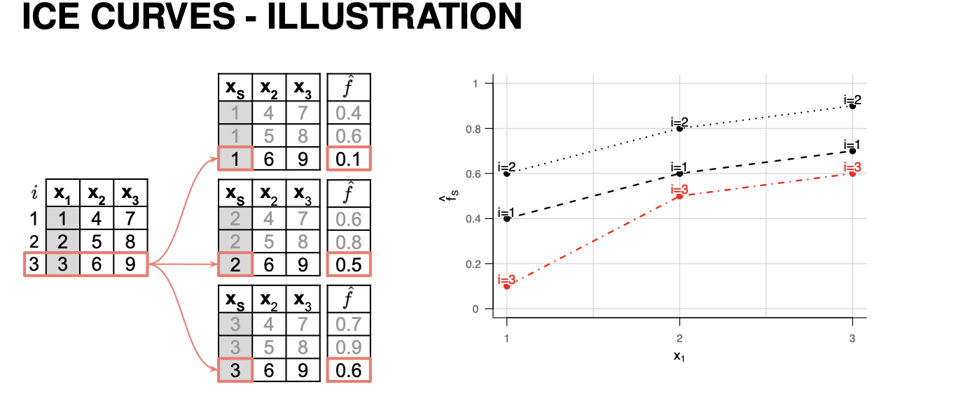
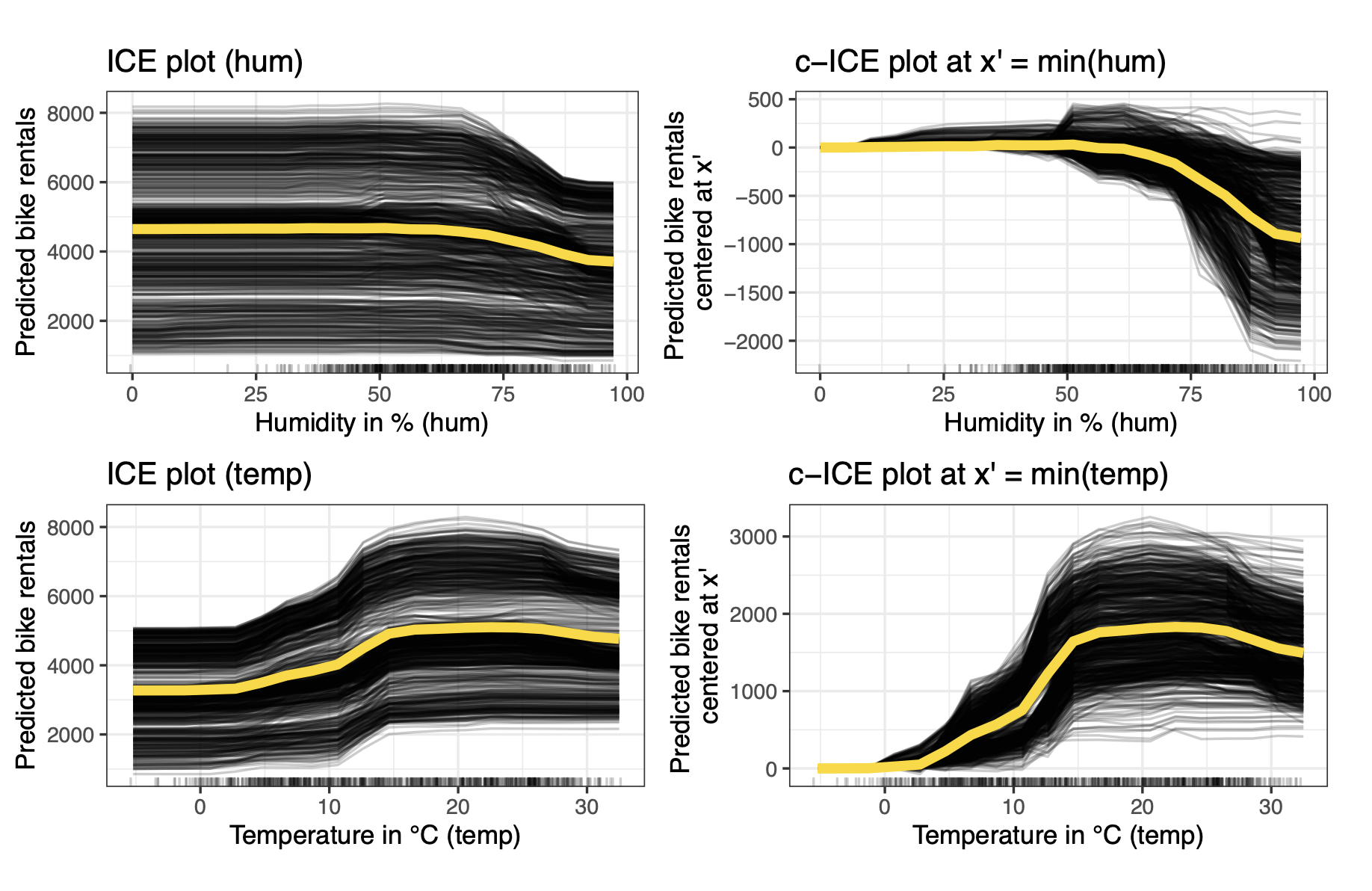
- Each line in an ICE plot represents how the prediction for a single specific instance changes as the feature of interest $x_S$ is varied. ICE curves provide a local view, showing the feature’s effect for that specific observation.
- If the ICE curves for different observations are parallel, it suggests a homogeneous effect of the feature across observations. Conversely, if the curves have different shapes or slopes, it indicates heterogeneous effects, possibly due to interactions between $x_S$ and other features. For example, in a bike-sharing dataset, parallel ICE curves for temperature would mean the effect of temperature on bike rentals is similar for all days, while diverging curves might show that temperature’s effect changes based on other factors like humidity or season
§3.03: Partial Dependence (PD) Plot
Partial Dependence Plots (PDPs) are a model-agnostic method that visualizes the average marginal effect of one or two features on the predicted outcome of a machine learning model. They provide a global interpretation by showing how, on average, the model’s prediction changes as the feature(s) of interest vary, while averaging out the effects of all other features
-
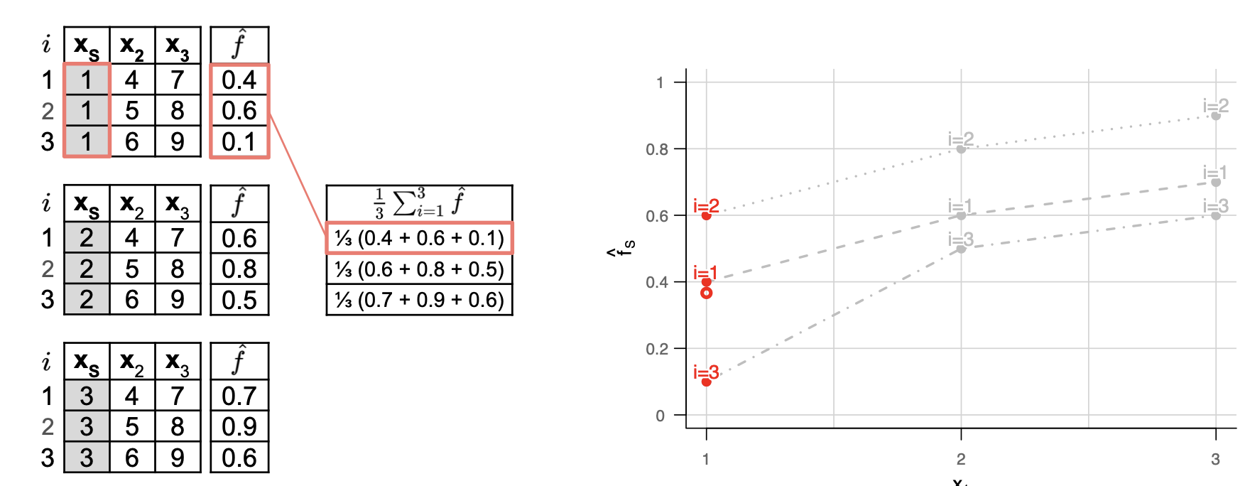
The PD function is formally defined as the expectation of the model’s prediction $\hat{f}(x_S, x_{-S})$ with respect to the marginal distribution of features not in $S$ i.e. ($-S$).
\[f_{S, PD}(x_S) = E_{x_{-S}}[\hat{f}(x_S, x_{-S})] = \int_{- \infty}^\infty \hat{f}(x_S, x_{-S}) d P(x_{-S})\] -
Normally, this is estimated using the grid-values generated by averaging the ICE-curves point-wise. \(\hat{ f_{S, PD}(x_S)} = \frac{1}{n}\sum_{i=1}^n \hat{f}(x_S, x_{-S})\)
Example
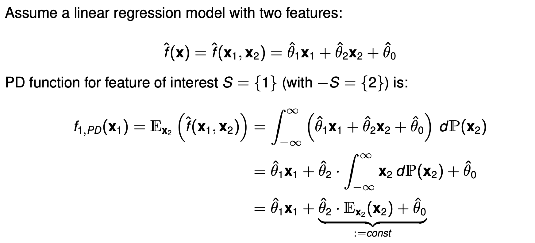
- An important thing to note as to why $\int \hat{\theta_1}x_1 dP(x_2) \neq \hat{\theta_1}x_1 x_2 $. It is because integrals wrt to the distribution works a bit differently: $$ \int \hat{\theta_1}x_1 dP(x_2) = \hat{\theta_1}x_1 \int 1 . dP(x_2) $$
- This is not integrating with respect to the variable $x_2$ (like $d x_2$) in the calculus sense. It’s taking the weighted average of the function over the probability distribution $P(x_2)$. Therefore it is the Expected value of function under a probability distribution i.e. $ E_{x_2}[\theta_1 x_1] $ which is simply $ \theta_1 x_1$ as it is not a random variable wrt $x_2$.
- When features are correlated, the process of creating artificial data points for ICE and PDP calculations can lead to unrealistic combinations of feature values. When calculating the effect of $x_1$, PDP will average over the full marginal distribution (or full grid if using equidistant sampling) of $x_2$ which can create many unrealistic combinations (like temperature being -1 and season being summer).
- PDP would include many such unrealistic combinations and models may behave strangely when making predictions for data points far outside the manifold of the training data.
- Consequently, the resulting PDP or ICE curves might reflect these unreliable predictions from extrapolated regions, potentially leading to misleading interpretations of the feature’s true effect within the realistic data distribution.
- This is even more problematic for overfitted or interaction-heavy models.
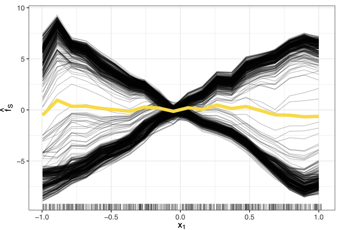
PDP plots average ICE curves and thus may obscure heterogenous effects. Therefore it is important to plot both the ICE curves and the PDP together to detect these.
Centered ICE PLots
-
Centered Individual Conditional Expectation (c-ICE) plots are a visualization technique used to enhance the interpretability of standard ICE plots, particularly when trying to discern heterogeneous effects or interactions between features. They address a common issue with regular ICE plots where differences in the starting prediction levels (intercepts) for various instances can make it difficult to compare the shapes of the individual curve.
-
Simply centering them at a fixed reference point solves the issue. Often $x’= \min (x_S)$ is used. \(\hat{f}_{S, cICE}(x_S) = \hat{f}(x_S, x_{-S}^{(i)}) - \hat{f}(x', x_{-S}^{(i)}) = \hat{f}^{(i)}(x_S) - \hat{f}^{(i)}(x')\)
§3.04: Marginal Effects
Marginal effects (MEs) quantify changes in model predictions resulting from changes in one or more features. They are particularly useful when parameter-based interpretations (like coefficients in linear models) are not straightforward due to model complexity or interactions.
There are two main ways to compute marginal effects:
- Derivative Marginal Effects (dMEs): These are numerical derivatives representing the slope of the tangent to the prediction function at a given point. They require the model to be differentiable (and therefore fails for stepwise models like Tree Ensembles, RuleFit, etc) and provide a rate of change of the prediction with respect to the feature value.
- Forward Marginal Effects (fMEs): These use finite forward differences, i.e., the difference in predictions when the feature is increased by a small step $h$. This approach does not require differentiability and works for any model and feature type.
Both methods measure the local effect of a feature on the prediction, but they differ in their assumptions and robustness.
Derivative Marginal Effects (dMEs)
-
Definition: The derivative marginal effect of feature $x_j$ at point $x$ is the partial derivative of the prediction function $f$ with respect to $x_j$:
\[dME_j(x) = \frac{\partial \hat{f}(x)}{\partial x_j} \approx \frac{\hat{f}(x_1,..,x_j+h_j,..,x_p) - \hat{f}(x_1,..,x_j -h_j,..,x_p)}{2 h_j}\] - Interpretation: It represents the instantaneous rate of change in the prediction when $x_j$ changes by an infinitesimal amount, holding other features fixed.
- Requirements: The prediction function must be differentiable with respect to $x_j$. This can fail for models with non-smooth prediction surfaces, such as decision trees.
- Limitations: In the presence of non-linearity (i.e. based on the curvature the tangent function may overshoot or undershoot) or kinks in the prediction function, the tangent slope may misrepresent the actual change in prediction over a finite step.
Forward Marginal Effects (fMEs)
-
Definition: The forward marginal effect of feature $x_j$ at point $x$ with step size $h$ is:
\[fME_j(x, h_j) = \hat{f}(x_1,...,x_j + h_j,...,x_p) - \hat{f}(x)\] - Interpretation: It measures the exact change in the predicted outcome when $x_j$ is increased by $h$, holding all other features fixed.
- Advantages: Applicable to any model, including non-differentiable ones; Robust to kinks, plateaus, and step-wise changes in the prediction function; Provides an exact finite change rather than an approximation.
- Caveats: : The effect depends on the choice of step size $h$, and it is not scale-invariant (halving $h$ does not necessarily halve the effect)
ME for Categorical Features
Traditionally a reference category was fixed, and the ME was calculated by keeping all other features constant except changing the category. The definition for fME mirrors the continuous equivalent:
\[fME_j(x; x_j^{new}) = \hat{f}(x_j^{new}, x_{-j}) - \hat{f}(x_j, x_{-j})\]More on Marginal Effects
Local Instantiations
- ME (at $x^{(i)}$): Individual, observation-specific “what-if” effect.
- MEM (at mean $\bar{x}$): Effect at artificial profile (“average observation”).
- MER (at representative value): Effect at a user-defined profile.
Average Marginal Effect (AME)
-
It captures the global overall effect is simply the average of marginal effects across all individual observations. You can use fME or dME (formula below is for fME)
\[AME_s = \frac{1}{n} \Sigma_{i=1}^n [\hat{f}(x^{(i)}_s + h_s, x^{(i)}_{-s}) - \hat{f}(x^{(i)})]\] - They work for GLMs (like linear, logistic, poisson, etc) as the link function is often monotonic so the direction of the effect is stable. Because the effect direction is stable, averaging the marginal effects across all observations yields a meaningful global summary.
- They however fail for non-parametric methods because AMEs assume a consistent effect across the feature space.
- Non-parametric models can capture complex, non-linear relationships and high-order interactions that GLMs cannot. They don’t have a linear structure and can model complex, non-linear relationships.
- Therefore the effect of a feature can vary significantly across the feature space, depending on the values of other features. Averaging the marginal effects can obscure important heterogeneities, leading to misleading conclusions.
- AMEs assume a consistent effect across the feature space. Averaging these effects can result in an AME close to zero, even if the feature has a strong effect in specific regions
- Instead for non-parametric methods, instead local MEs should be examined. Instead of averaging, examine the distribution of marginal effects across the dataset. Moreover we should quantify the degree of non-linearity to understand how much the feature’s effect deviates from a simple linear relationship
Why MEs are Still meaningful
MEs provide a single scalar number to quantify the effect. Simultaneously perturbing multiple features still yields a scalar. Moreover it is captured at the actual data point and captures interactions without any assumptions, provides a non-linearity measure and is computationally cheap.
§3.05: Accumulated Local Effect (ALE) Plot
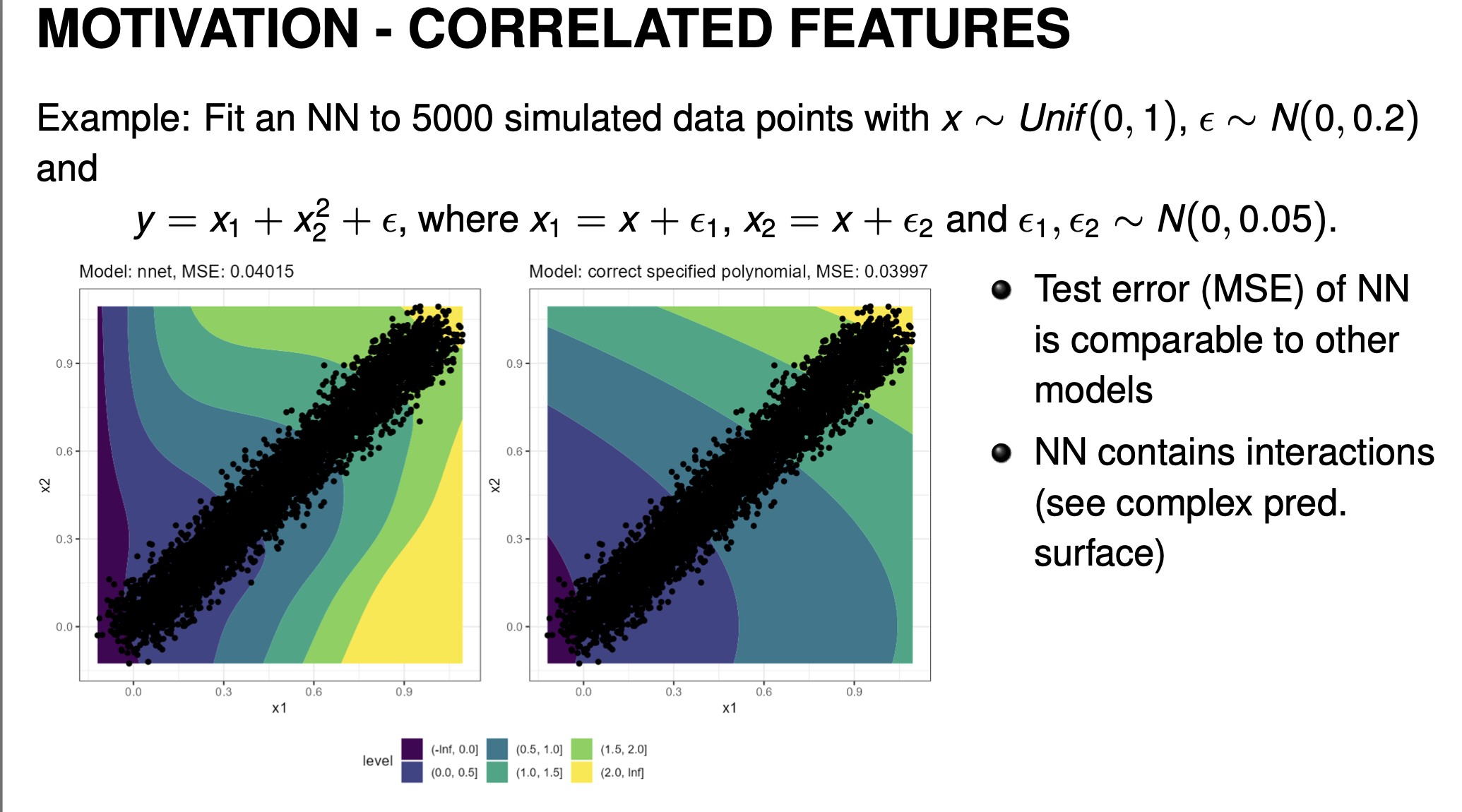
- Recall that PDP will average over the full marginal distribution (or full grid if using equidistant sampling). For a highly-correlated data, this could end up with PDP averaging over many unrealistic combinations which can lead to biased/misleading interpretations. Consider the following example:
-
Compare a neural network vs a correctly specified polynomial model to fit the above data. Although both have similar performance, note that the prediction surface for the neural network looks very different from the correctly specified quadratic. The neural network will still give predictions in the outside regions but may behave somewhat strangely. This is common for neural networks since they are highly complex and allow for the model to learn complex relations within the data distribution.
-
It is important to note that PD plots aren’t wrong. PD Plots describes the feature effect that the model estimated. Since the model also makes predictions for out-of-distribution data, the feature effects captured here reflect that. However if our interest is to interpret the feature effects of the data distribution, then PDP is the wrong tool. PD Plots give us an estimation of the feature effect that is true to the model, not the data.
M-Plots
-
One might argue that we look at a neighbourhood of the points instead of the full marginal aka the conditional distribution, then that should suffice and give us the feature effect present in the data:
\[E_{x_2|x_1}(\hat{f}(x_1, x_2)|x_1) \approx \hat{f}_{1,M}(x_1) = \frac{1}{|N(x_1)|} \Sigma_{i \in N(x_1)} \hat{f}(x_1, x_2)\]Where $N(x_1)$ is the index of all points within a fixed distance.
-
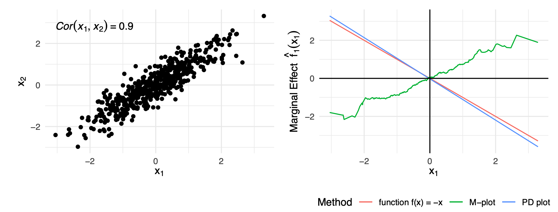
However, this creates an omitted variable bias. When we condition on $x_1$, we’re not isolating its pure effect. We’re capturing the combined effect of $x_1$ and all features that are correlated with it.When we fix $x_1=c$ and look at nearby observations, we’re implicitly also constraining $x_2$ to values around $E[x_2 \mid x_1 = c]$. This leads strange results. Imaging you have \(\hat{f}(x_1, x_2) = -x_1 + 2x_2\) where \(\rho(x_1, x_2) = 0.9\) but no interactions. Then it is very obvious that the feature effect for \(x_1\) should be a line with slope \(-1\). However, when calculating the m-plot, by taking the conditional distribution, we implicitly also model the effects of \(x_2\) which leads to the m-plot having a positive slope.
ALE Plots
-
ALE attempts to solve this problem by taking partial derivatives (local effects) of prediction function w.r.t. feature of interest and integrating (accumulate) them w.r.t. the same feature. This results in properly recovering the main effect of \(x_1\) alone.
Example
Consider $ \hat{f}(x_1, x_2) = 2x_1 + 2x_2 - 4x_1 x_2 $. Then $ \frac{\partial \hat{f}(x_1, x_2) }{\partial x_1} = 2 - 4x_2 $. Integrating this with respect to $x_1$ again yields $ \int_{z_0}^x \frac{\partial \hat{f}(x_1, x_2) }{\partial x_1} d x_1 = [2x_1 - 4x_1 x_2]_{z_0}^x$ which completely recovers the main effect w.r.t $x_1$ - The Accumulated Local Effects (ALE) is then calculated using the following steps:
- Estimate Local Effects \(\frac{\partial\hat{f}(x_S, x_{-S})}{\partial x_S}\) evaluated at certain points \((x_S = z_S, x_{-S})\). The use of Partial Derivates here leads to completely removing the main effects of \(x_{-S}\).
- Averaging Local Effects: The local effects are averaged over the conditional distribution \(\mathbb{P}(X_{-S} \mid x_S)\) which solves the extrapolation issues.
- Integrate Averaged Local Effects: Accumulates local effects to estimate global main effect. The integration here recovers the main effect of \(x_S\) solving the OVB issue of M-Plots.
-
The Uncentered first oder ALE \(\tilde{f}_{S, ALE}(x)\) is defined as:
\[\tilde{f}_{S, ALE}(x) = \int_{z_0}^x \mathbb{E}_{x_{-S}\mid x_S}(\frac{\partial\hat{f}(x_S, x_{-S})}{\partial x_S} \mid x_S = z_S) dZ_s\] -
Subtracting the average of the uncentered ALE yields the centered ALE with zero mean:
\[f_{S, ALE}(x) = \tilde{f}_{S, ALE}(x) - \int_{-\infty}^\infty \tilde{f}_{S, ALE}(x_S) d \mathbb{P}(x_S)\] -
Many models are not differentiable so in practice, the partial derivatives are approximated by finite differences of the predictions within K intervals of \(x_S\). A simple way to create these intervals is by using the quantile distributions.
Example
Let's use the bike sharing dataset example, where we have a model that predicts the number of rented bikes based on features like temperature, humidity, and windspeed. We want to understand the local effect of temperature using interval-based finite differences.- Partition the Temperature Feature: Suppose the temperature in our dataset ranges from 0°C to 40°C. We partition this range into 40 intervals of 1°C each: $ [0,1),[1,2),…,[39,40)$.
- Calculate Finite Differences for an Interval: Let's focus on the interval $[20°C, 21°C)$: First, we identify all data points in our dataset where the recorded temperature is between 20°C and 21°C. Let's say we find an observation, $obs_A$, with the following features, temp = 20.5, humidity = 60%, windspeed = 15. To calculate the finite difference for $obs_A$, we keep its other features (humidity and windspeed) fixed and create two new data points by replacing the temperature with the interval's boundaries (temp = 20, and temp = 21). Suppose $\hat{f}(21, 60, 15) = 4200$ and $\hat{f}(20, 60, 15) = 4150$, then the finite difference $\Delta^{(A)}_{temp, [20,21)} = 4200-4150 = 50$.
- The process of calculating the finite difference is repeated for every data point that has a temperature falling within the [20°C, 21°C) interval. Since each of these data points has a unique combination of other features (like humidity and windspeed), the calculated local effect will vary for each one.
- These individual finite differences are then averaged to get a single, stable estimate of the local effect for that interval : $\bar{\Delta}_{temp, [20,21)} = \frac{1}{\mid x_{temp}^{(i)} \in [20,21) \mid} \sum_{x_{temp}^{(i)} \in [20,21) } \Delta^{(i)}_{temp, [20,21)}$
- The next step is to accumulate—or sum up—these average local effects across the intervals in sequence. This reconstructs the main effect of the temperature feature over its entire range : $$ \tilde{f}_{temp,ALE}(x) = \sum_{k=1}^{K} \bar{\Delta}_{temp, [k-1, K)} $$
- Finally, you can calculate the centered ALE $$ f_{temp,ALE}(x) = \tilde{f}_{temp,ALE}(x) - \frac{1}{n} \sum_{i=1}^n \tilde{f}_{temp,ALE}(x^{(i)}) $$
Differences between PD and ALE
| PD | ALE |
|---|---|
| Bivariate PD also captures the main effects along with interactions. | 2nd Order ALE only estimates pure interaction effects. |
| Averages over the marginal distribution of \(x_{-S}\). | Averages the change of predictions (approximated by finite differences) over the conditional distribution \(\mathbb{P}(X_{-S} \mid x_S = z_S)\) . |
| Prone to extrapolation by creating unrealistic data points if features are correlated. | ALE integrates partial derivatives of feature S over zS, isolating the effect of feature S and removing the main effect of dependent features. |
| Not centered; the plot shows the actual average prediction value. | ALE is centered so that \(E_{x_S}(f_{S, ALE}(x)) = 0\). |
| Computationally expensive, requiring \(n*g\) predictions (where \(g\) is the number of grid points). | Computationally more efficient, as you only need to compute two predictions for each observation. |