Chapter 6: Local Interpretable Model-agnostic Explanations (LIME)

A common approach to interpret an ML model locally is implemented by LIME. The basic idea is to fit a surrogate model while focussing on data points near the observation of interest. The resulting model should be an inherently interpretable one.

§6.01: Introduction to Local Explanations

TO-DO

§6.02: Local Interpretable Model-agnostic Explanations (LIME)

LIME (Local Interpretable Model-Agnostic Explanations) is a popular technique for explaining the predictions of any black-box machine learning model. Its primary objective is to provide local, human-understandable explanations for individual predictions, regardless of the underlying model type or complexity. LIME is called “model-agnostic” because it treats the original model as a black box, requiring no access to its internal structure, parameters, or training process. This universality makes LIME applicable to any machine learning model, from simple linear regression to complex deep neural networks.

LIME operates under a fundamental assumption of locality: while the complex model \(\hat{f}\) may exhibit highly non-linear behavior globally, it behaves in a relatively simple manner within small neighborhoods of any given instance \(x\). This local simplicity can be effectively approximated using an interpretable surrogate model \(\hat{g}\). The surrogate model \(\hat{g}\) is intentionally chosen to be simple and interpretable—typically a linear regression or shallow decision tree. The key requirement is that \(\hat{g}\) should be both interpretable to humans and faithful to the original model’s behavior locally.
LIME generates synthetic inputs \(z\) in the neighborhood of the instance \(x\) being explained. The concept of “closeness” or “neighborhood” is captured using a proximity measure \(\phi_x(z)\), which assigns higher weights to synthetic samples that are closer to the original instance \(x\). The goal is to ensure that \(\hat{g}(z) \approx \hat{f}(z)\) for synthetic inputs \(z\) near \(x\).
LIME formulates the explanation problem as an optimization task that balances two competing objectives:
1. Local Fidelity: Minimize the loss \(L(\hat{f}(z), \hat{g}(z))\) (such as \(L_2\) loss) between the original model’s predictions and the surrogate model’s predictions on synthetic data. The overall local fidelity objective is measured by a weighted loss:
\[L(\hat{f}, \hat{g}, \phi_x) = \sum_{z \in Z} \phi_x(z) L(\hat{f}(z), \hat{g}(z))\]
1. Interpretability: Minimize the complexity of the surrogate model \(\hat{g}\), measured using a complexity measure \(J\) (such as the \(L_0\) norm)
The final objective seeks to find a surrogate model \(\hat{g}\) that is minimally complex yet maximally faithful in the local neighborhood of the instance being explained:
\[\operatorname{argmin}_{\hat{g} \in G} L(\hat{f}, \hat{g}, \phi_x) + J(\hat{g})\]

LIME Algorithm

For a pre-trained black-box model \(\hat{f}\), observation \(x\) whose prediction we wish to explain, and an interpretable model class \(G\):

Independently sample new points \(z \in Z\) by slightly modifying the features of the selected instance. For tabular data, this might mean sampling from the feature’s distribution; for images, it could mean turning superpixels on or off; for text, removing or replacing words.
Retrieve prediction \(\hat{f}(z)\) for obtained points \(z\) from the black-box model.
Calculate the weights for \(z \in Z\) by their proximity measure \(\phi_x(z)\) to quantify closeness to \(x\).
Train interpretable surrogate model \(\hat{g}\) on data points \(z \in Z\) using weights \(\phi_x(z)\) and \(\hat{f}(z)\) as targets.
Return \(\hat{g}\) as the local explanation for \(\hat{f}\).

§6.03: LIME Examples

TO-DO

§6.04:LIME Pitfalls

While LIME is a powerful and intuitive tool for explaining the predictions of complex “black-box” models, it’s crucial to understand its limitations to use it responsibly as its methodology gives rise to several significant challenges.

1. Sampling: Ignoring Feature Dependencies and Extrapolation Risks

LIME normally generates perturbations by sampling each feature independently from a univariate distribution. This is a strong assumption on the data distribution breaking correlation structures and feature dependencies. For example LIME could generate a synthetic data point for a person with height 7 feet and weight 50kg - a highly unrealistic combination. By ignoring these dependencies, LIME evaluates the model on data points that are unlikely or impossible to occur naturally.
These unrealistic data points could lie very far from actual data distribution and the black-box model may perform very poorly in these extrapolated regions. The surrogate model which which uses the output of the black-box models as ground-truth could then yield an interpretable yet non-sensical model.
Solutions: Sample locally from the true data manifold (challenging in high-dimensional or mixed-type settings) or restrict sampling to training data in the neighbourhood (requires enough training points).

2. Locality Definition: Sensitivity to Kernel Width and Distance Metrics

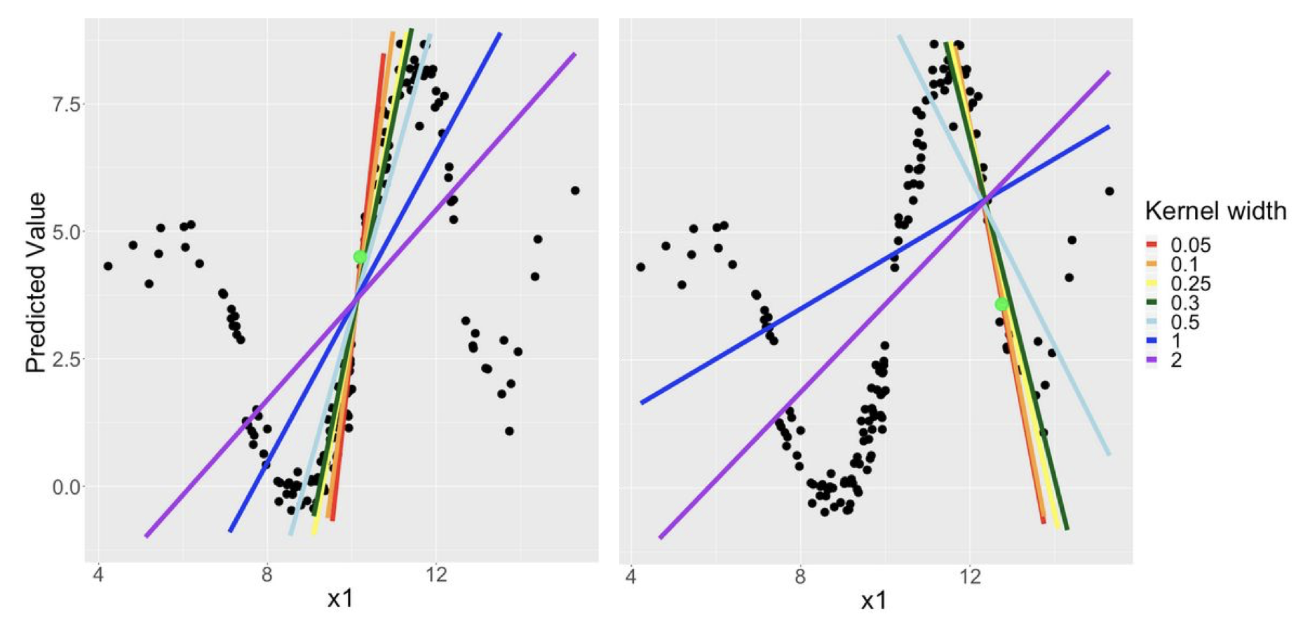
LIME’s explanations are highly dependent on the definition of “locality,” which is controlled by a kernel function that assigns weights to the generated samples based on their proximity to the instance being explained
The kernel width (or bandwidth) determines the size of the neighborhood around the instance of interest. A small kernel width creates a very small, focused neighborhood, while a large one considers a wider region. This choice presents a trade-off: a smaller neighborhood might be easier to approximate with a linear model but may be less stable/more noisy/overfit the noise, while a larger one might smooth over important local complexities. Explanations can be significantly altered simply by changing the kernel width, making them potentially unreliable if the width is not chosen carefully.

The choice of distance metric used within the kernel function also influences the explanation. Different metrics can result in different neighborhoods and, consequently, different explanations. The performance and fairness of comparisons between explanations can be affected by the choice of distance metric and its interaction with the kernel width.
Solutions: We could use Gower distance directly as weights instead of using kernels, but this results in distant points still receiving high weights causing the explanations to be more global than local. s-LIME adaptively selects the kernel width to balances the fidelity and stability.

3. Local vs. Global Features: Overshadowing of Local Signals

LIME is designed to answer the question: “Why did the model make this specific prediction for this particular instance?” It achieves this by focusing on local fidelity, creating a simple explanation that is true in a small neighborhood around the point of interest.
Many machine learning models are dominated by features with strong global importance—features that have high predictive power across the entire dataset. When LIME builds its local, sparse linear model, it often selects the features that best approximate the black-box model’s behavior in the local sample. If a feature has a powerful global effect, its signal is likely to be strong even in the local neighborhood.
The pitfall is that LIME might select these globally important features for the local explanation, even if other, less globally-powerful features are the true drivers for the specific prediction. The strong “global accent” of a feature can drown out the more subtle “local dialect” that genuinely explains the instance. The resulting explanation becomes less about the local reasons and more a reflection of the model’s overall behavior.
Consider a model that predicts the price of apartments. Across the entire city, the most important feature is square_footage. However, for a small, 500 sq. ft. penthouse apartment with a panoramic view of the city skyline, the feature has_panoramic_view is the actual reason for its exceptionally high price. When we use LIME to explain the price of this specific penthouse, the algorithm samples points around it. For all these perturbed points, the square_footage feature will still have a strong influence on the model’s output because it’s a globally dominant feature. As a result, LIME’s explanation might report that square_footage is a significant (and positive) contributor to the price, which is confusing and misleading for this small apartment. The truly decisive local feature, has_panoramic_view, might receive a lower importance score or be excluded entirely if the explanation is forced to be sparse, because its strong effect is limited to a very small subset of luxury properties.

4. Poor Fidelity for Complex Models

While many complex functions are locally linear, this is not always the case. If the decision boundary of the black-box model has high curvature even in a small neighborhood, a linear surrogate model will be a poor approximation.
A very simple surrogate model will have low fidelity but unreliable explanations. On the other hand a complex surrogate model will have high fidelity but may be difficult to interpret.

5. Hiding Biases

LIME samples out-of-distribution (OOD) points, making it exploitable and developers can adversarially hide bias in the original model. LIME can be fooled if explanations rely on model behavior outside the true data manifold.
Since LIME is a model-agnostic method that only queries the model for predictions, it can be gamed. A malicious actor could design a biased model that appears fair when inspected with LIME. This is a form of adversarial attack on interpretability methods. The model could be trained to make discriminatory predictions based on a sensitive feature (e.g., race or gender) but is also carefully designed to provide plausible, non-discriminatory explanations whenever it is audited.

LIME explains the model’s output, not its internal reasoning, so it can be fooled by a model that has learned to “lie” convincingly.
A user with malicious intent could experiment with different kernel widths or sampling strategies until they find a setting that produces a more favorable—but ultimately misleading—explanation. For instance, they could generate an explanation that downplays the model’s reliance on a sensitive feature like race or gender.

6. Robustness: Unstable Explanations for Similar Points

A critical flaw in LIME is its lack of robustness. Small, sometimes imperceptible, changes to the input instance can lead to dramatically different explanations. This instability can stem from two sources:
1. The sampling process: Since LIME relies on random sampling to create the neighborhood, different runs (with different random seeds) can produce different sets of perturbed points and thus different explanations.
2. The model’s decision boundary: If the black-box model has a very complex and irregular decision boundary, two points that are very close together might fall on different sides of a local “wrinkle,” leading to very different linear approximations.
Using LIME can be like measuring with a ruler made of elastic. If you measure the same object twice and get different results, you can’t be confident in either measurement. An explanation method should be reliable and consistent, but LIME can fail this test.

7. Superpixels (for Images): Instability from Segmentation

When applying LIME to images, it’s not feasible to perturb individual pixels. Instead, LIME first segments the image into a set of “superpixels” (contiguous patches of similar pixels). The explanation is entirely dependent on the initial, arbitrary segmentation method. Different segmentation algorithms, or even different parameters for the same algorithm, will produce different superpixels. This, in turn, will lead to different explanations for the same image, model, and prediction.