Chapter 8: Feature Importance

Methods belonging to this category aim to rank the features according to their influence on the predictive performance of an ML model. Depending on the interpretation goal, these methods are more or less suitable."

§8.01: Introduction to Loss-based Feature Importance

Whilst Feature effects describe the relationship of features \(x\) with the prediction \(\hat{y}\), Feature Importance methods quantify the relevance of features w.r.t. prediction performance and provides insight into the relationship with \(y\).
Many loss-based feature importance methods exist and they mainly differ in
1. How they remove/perturb the feature of interest \(X_j\) : This can be done by removing and refitting the model, or replacing it with \(\tilde{X_j}\) which is sampled from the marginal/conditional, or by marginalizing out \(X_j\).
2. How they compare model performance before/after feature removal: This can be done by measuring drop in performance when \(X_j\) is dropped (backward feature elimination), or by gain in performance when \(X_j\) is added to an empty model (forward feature selection), or by comparing across different feature sets like Shapely.

§8.02: Permutation Feature Importance (PFI)

Goal: Assess how important features are for predictive performance of a fixed trained model \(\hat{f}\) on a given dataset \(\mathcal{D}\).
Idea: “Destroy” feature of interest \(X_S\) by perturbing it in such a way that it becomes uninformative and then estimate change in model performance.
Question: \(X_S\) cannot be made uninformative by removing it from the model as retraining without \(X_S\) gives a different model.
Solution: Simulate feature removal by replace \(X_S\) with a perturbed version \(\tilde{X_S}\) that is independent of \((X_{-S}, Y)\) by preserves the marginal distrubtion \(P(X_S)\). Adding random noise distorts the marginal, instead if you permute it, it preserves the marginal and breaks the dependence with \(Y\).
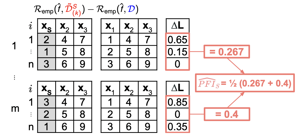
\[PFI_S = \mathbb{E}[L(\hat{f}(\tilde{X_S}, X_{-S}), Y)] - \mathbb{E}[L(\hat{f}(X), Y)]\]
A sample estimator using independent test set \(\mathcal{D} = \{ (x^{(i)}, y^{(i)}) \}_{i=1}^n\) can be derived. Repeat \(m\) times and calculate the average:
1. Perturb the feature values for \(X_S\) and create \(\tilde{\mathcal{D}}^S\) with the perturbed feature \(\tilde{X_S}\) in place of \(X_S\).
2. Make predictions using \(\tilde{\mathcal{D}}^S\) and \(\mathcal{D}\).
3. Compute the loss for each observation and aggregate it.

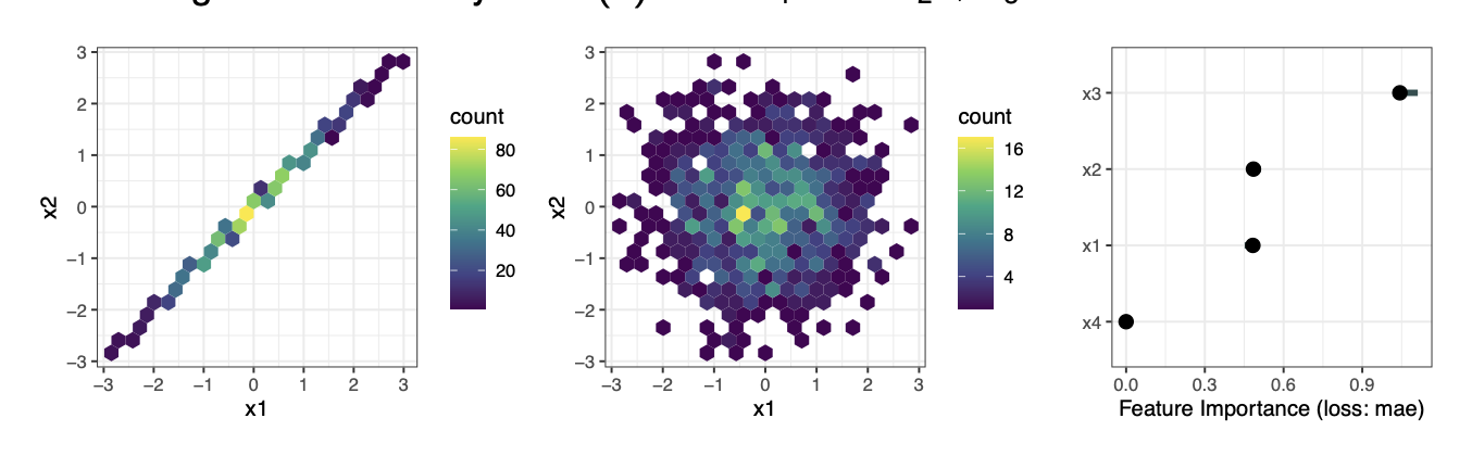
Permuting features despite correlations/dependence with other features can lead to unrealistic combinations of feature values leading to extrapolation issues (i.e. the fitted model is not really fit for predicting out of distribution data and can cause very weird outputs).

Permuting \(x_j\) also destroys any interactions it has with other features. Therefore PFI score contains importance of all interactions with the permuted feature.
Interpreting PFI depends on whether training/test data is used. PFI on train data highlights features that model overfits to. These spurious feature-target dependencies vanish on test. Therefore to identify features that help model to generalize, compute PFI on test data.

Testing Importance (PIMP)

The main idea behind PIMP is to test if an observed \(\hat{PFI}_j^{obs}\) score is significantly greater than expected under the \(H_0\) of \(X_j\) being not important i.e. \(H_0:\) Feature \(X_j\) is conditionally independent of \(y\).
Approximate null distribution of PFI scores under \(H_0\) by repeated permuting \(y\) as it breaks relationships to all features and PFI scores reflect the noise. Now you can assess the significance of PFI scores via tail probability under \(H_0\) and use this as a feature importance score
The algorithm is given below
1. For \(b \in \{1,...,B\}\): Permute \(y\), retrain model on \((X, y^{(b)})\). Compute \(\hat{PFI}_j^{(b)}\) for each feature \(j\)
2. Train the model on original data \((X, y)\)
3. For each feature \(j \in \{1,...,p\}\), compute \(\hat{PFI}_j^{obs}\) with unpermuted \(y\). Fit a probability distribution to \(H_0\) scores and compute the p-value.
  - Parametric: \(\mathbb{P}(\hat{PFI}_j^{(m)} \geq \hat{PFI}_j^{obs})\)
  - Non-Parametric: \(p_j = \frac{1}{B} \sum_{b=1}^B \mathbb{I}[\hat{PFI}_j^{(b)} \geq \hat{PFI}_j^{obs}]\)

§8.03: Conditional Feature Importance (CFI)

PFI not only breaks association between \(X_S\) and \(y\), it also breaks association between \(X_S\) and \(X_{-S}\) i.e. \(\mathbb{P}(X_S, X_{-S}) \neq \mathbb{P}(\tilde{X_S}, X_{-S})\) leading to issues when extrapolating.
CFI instead replaces \(X_S\) with perturbed \(\tilde{X_S}\) such that the joint distribution between the features is preserved but the association with the target \(y\) is broken i.e. \(\mathbb{P}(X_S, X_{-S}) = \mathbb{P}(\tilde{X_S}, X_{-S})\) and \(\tilde{X_S} \perp \!\!\! \perp y\)
This can be done for example by conditionally perturbing features

§8.04: Leave One Covariate Out (LOCO)

Learn a model \(\hat{f}_{-j}\) on \(\mathbb{D}_{train, -j}\) and compute the \(L_1\) loss difference for each sample in \(\mathbb{D}_{test}\)
\[\Delta_j^{(i)} = \mid y^{(i)} - \hat{f}_{-j}(x^{(i)}) \mid - \mid y^{(i)} - \hat{f}(x^{(i)}) \mid\]
The LOCO is then \(med(\Delta_j^{(i)})\). If you instead use the mean then it is simple comparing the empirical risk - \(R_{emp}(\hat{f}_{-j}) - R_{emp}(\hat{f})\).
Whilst it is easy to implement, it doesn’t provide insight into a specific model (only the learner). Furthermore model training is often stochastic and noisy so refits are not the best solution. They are also computationally intensive.