Chapter 11: Advanced Risk Minimization

This chapter revisits the theory of risk minimization, providing more in-depth analysis on established losses and the connection between empirical risk minimization and maximum likelihood estimation.

§11.01: Risk Minimisers

• Our goal is to minimise the risk, for a certain hypothesis $f \in H$ and loss $L(y, f(x))$

  \[R_L(f) = E_{xy}[L(y,f(x))] = \int L(y,f(x))\text{dP}_{xy}\]

  This risk here is simple what I have previously known as “loss”. $f \in H$ is a just a possible model (like logistic, linear, etc) and we sum over all $x,y$. We simply want to minimize the expectation with respect to the data generating process.

• In an ideal world, the hypothesis space $H$ is unrestricted i.e. $f$ can take any arbitrary form (no restrictrictions like the linear model, etc). We also assume that Risk Minimisation can be solved perfectly and efficiently and that we know the data generating process $\text{P}_{xy}$. How should $f$ be chosen?

• The $f^* \in H$ with minimal risk is called the Risk Minimiser, Population Minimizer, or Bayes Optimal Model where

  \[f^* = \underset{f: X \rightarrow \mathbb{R}^g}{\operatorname{argmin}} R_L(f) = \underset{f: X \rightarrow \mathbb{R}^g}{\operatorname{argmin}} \int L(y, f(x)) \text{dP}_{xy}\]

  The resulting risk is called the Bayes Risk,

  \[R_L^* = \inf R_L(f)\]
• If $f \in H$ is truly unrestricted, then we choose an $f$ such that $f(x) = y \text{ } \forall x \in X$ Or more generally, we can construct an $f$ such that $f(x) = c$ where $c$ is any value we want that minimizes the risk i.e. we can construct a pointwise optimizer.

• In practice, (i) we usually have to restrict the hypothesis space such that we can efficiently search over it (ii) we usually do not also know the true data generating process $\text{P}_{xy}$. Instead of $R_L(f)$ (aka the theoretical risk minimiser), we usually optimise the empirical risk i.e.

  \[\hat{f} = \underset{f \in H}{\operatorname{argmin}}R_{emp} (f) = \underset{f \in H}{\operatorname{argmin}} \Sigma_{i=1}^n L(y^{(i)}, f(x^{(i)}))\]

  According to Law of Large Numbers, $R_{emp} \rightarrow R_L(f)$ as $n \rightarrow \infty$. (This is basically loss as I have always learnt).

• The goal of learning is there to minimise the Bayes Regret i.e. train a model such that the difference between $R_L(\hat{f}) - R_L^*$ is as low as possible. Note that this Bayes Regret can be decomposed as follows:

  

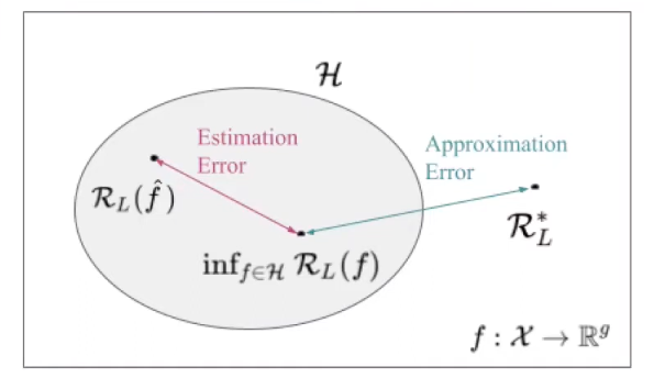
  (i) Estimation Error: We fit $\hat{f}$ via the empirical risk minimization and usually use approximate optimisation. Therefore we do not find the optimal $f \in H$. In simple words given that we have restricted the Hypothesis space, we can still only find the empirical risk minimiser since the true data generating process is not known. The Estimation error identifies this delta.

  (ii) Approximation Error: Now even if we find the optimal model when restricting the hypothesis space (i.e. we know the data generating process and its not an empirical estimation - note how its $f$ and not $\hat{f}$), it is still entirely possible that that the bayes optimal model is not even in our hypothesis space (For example if the true optimal model is quadratic but the hypothesis space is linear). The approximation error accounts for this error.

(Universally) Consistent Learners

• Consistency is an asymptotic property of a learning algorithm, which ensures the algorithm returns the correct model when given unlimited data

• If we study the risk $R$ of our inducing algorithm $I$ for a specific data generating distribution $P_{xy}$, and we sample training sets $D_{train}$ from this distribution of size $n_{train}$ and we run the algorithm on $D_{train}$, and evaluate the true risk of the model, in probability the risk converges to Bayes Risk $R_L^*$, we say that the learning method $I$ is consistent wrt to $P_{xy}$.

  \[R(I(D_{train}), \lambda) \rightarrow^p R^*_L\]
• Since we usually do not know $P_{xy}$, consistency is often not useful to choose a learning algorithm. A more interesting concept is Universal Consistency: An algorithm is universally consistent if it is consistent for any distribution.
• Whilst Universal Consistency is a desirable property, it does not tell us anything about convergence rates i.e. how efficiently the algorithm works under a limited amount of data. It is a limited property as the training size goes to infinity.

Optimal Constant Models

• While the risk minimizer gives us the (theoretical) optimal solution, the optimal constant model (i.e. featureless predictor) gives us a computable empirical lower baseline solution.

  The model $f(x) = \theta$ optimizes the risk $R_{emp}(\theta)$.

---

§11.02:Pseudo-Residuals

• In regression, the residuals are defined as $y - f(x)$. If we have partially fitted a model, the best point wise update is to move in the direction of the residual.

• We further define pseudo-residuals as the negative first derivates of loss functions wrt $f(x)$:

  \[\tilde{r} = -\frac{\partial L(y, f(x)) }{\partial f(x)}\]

  Consider $L(y, f(x)) = (y-f(x))^2$ i.e. the $L_2$ loss. Then, $\tilde{r} = 2(y-f(x))$

• Similarly, if we compute the best point-wise update using gradient descent,

  \[f(x) \leftarrow f(x) - \frac{\partial L(y, f(x))}{\partial f(x)} = f(x) + \tilde{r}\]

  Iteratively stepping in the direction of the pseudo-residuals is the whole idea behind gradient boosting.

• Normally, you don’t do gradient descent on the model itself (since then there is no restriction on the form of the model) as you may end up with an invalid model which does not lie in the hypothesis space. Thus gradient descent is normally performed on the parameters of the model:

  \[\theta^{[t+1]} = \theta^{[t]} - \alpha^{[t]} \nabla_{\theta}R_{emp}(\theta)|_{\theta = \theta^{[t]}}\]
• Since $R_{emp}(\theta) = \Sigma_{i=1}^n L(y^{(i)}, f)|_{f = f(x^{(i)}|\theta)}$ , (sum of losses); using the chain rule: \(\nabla_{\theta}R_{emp}(\theta) = \sum_{i=1}^n \frac{\partial L(y^{(i)}, f)}{\partial f}|_{f = f(x^{(i)}|\theta} . \nabla_{\theta}f(x^{(i)}|\theta) = - \Sigma \tilde{r}^{(i)}. \nabla_{\theta} f(x^{(i)}|\theta)\)
• Hence the update is very flexible, nearly loss-independent and is determined by:
  1. A loss-optimal directional change of the model output (the 1st term)
  2. A loss-independent derivative of f (the 2nd term)

---

§11.03: L2 Loss

Risk Minimiser

• The $L_2$ loss is given by $L(y, f(x)) = (y - f(x))^2$. Minimising this function is the same as minimising $0.5 (y - f(x))^2$. Considering this as our loss function, we get

  \[\frac{\partial L(y, f(x))}{\partial f(x)} = y - f(x) \Rightarrow \tilde{r} = r\]

  i.e. the pseudo-residuals are equal to residuals.

• Using the law of total expectation we get, \(R_L(f) = E_{XY}[L(y, f(x))] = E_X[E_{Y|X}[ L(y, f(X) | X = x ]] = E_X[E_{Y|X}[ (y-f(X))^2 | X=x ]]\)

• In a theoretical risk minimisation problem, we have an unrestricted hypothesis space and therefore we can construct an $f$ point-wise such that it outputs any value $c$. Hence we no longer need to consider the outer expectation over $X$. The problem then boils down to finding a $c$ such that $E_{Y\mid X}[(y-c)^2 \mid X = x]$ is minimum i.e.

  \[\hat{f}(x) = \underset{c}{\operatorname{argmin}} M(c) = E_{Y|X}[(y-c)^2 | X = x]\] \[\begin{aligned} M(c) &= \mathbb{E}_{Y|X}[(y - c)^2 \mid X = x] - \left(\mathbb{E}_{Y|X}[y \mid X = x] - c\right)^2 \\ &= \operatorname{Var}(Y - c \mid X = x) + \left(\mathbb{E}_{Y|X}[y \mid X = x] - c\right)^2 \\ &= \operatorname{Var}(Y \mid X = x) + \left(\mathbb{E}_{Y|X}[y \mid X = x] - c\right)^2 \end{aligned}\]

  Where we add a “0” and by definition $Var(X) = E[x] - E[x]^2$, and $Var(X+a) = Var(X)$, we get that that the first term (the variance) is independent of $c$ hence the optimization problem boils down to:

  \[\underset{c}{\operatorname{argmin}} (E_{Y|X}[Y|X=x] - c)^2\]

• It is evident that the function is minimum when $c = \hat{f}(X) = \mathbb{E}_{Y \mid X}[Y \mid X=x]$.

💡 Therefore, the risk minimiser for the L2 loss is the conditional expectation

Optimal Constant Model

• In the optimal constant model, $f(x) = \theta$, for the $L_2$ loss, $L(y, f(x)) = (y-\theta)^2$. Thus $R_{emp}(f; \theta) = \Sigma (y^{(i)} - \theta)^2$ . Thus taking the derivative of this function and setting it to 0 should give us the optimal $\hat{\theta}$.

  \[\frac{\partial R_{emp}(f; \theta)}{\partial \theta} = 2 \Sigma (y^{(i)} - \theta) =_{set} 0\] \[= \Sigma y^{(i)} - n\theta = 0 \Leftrightarrow \hat{\theta} = \frac{1}{n} \Sigma y^{(i)} = \bar{y}\]

• Note that in the L2 loss with optimal constant, we minimising the squared distances from one single point. In our case the mean. By definition, this is the sum of squared errors (just plug in $\bar{y}$ in the $R_{emp}$), which if divided by $n$ or $n-1$ is simply the empirical variance. Intuitively also this makes sense since in the optimal constant model we are minimising the squared distances from a single point.

💡 Under the optimal constant model, the optimal predictor is the empirical mean and the associated loss is the empirical variance. The same holds true for the point-wise construction / conditional distribution as seen in the previous section.

---

11.06: 0-1 Loss:

• Consider a discrete classifier $h(x): X \rightarrow Y$. The most natural choice for $L(y, h(x))$ would be the 0-1 loss:

  \[L(y, h(x)) = \mathbb{1}({y \neq h(x)})\]

  For the binary case, we can also express this as a scoring function $v = yh(x).$ Therefore the loss would then be $\mathbb{1}(v < 0).$ i.e. $\mathbb{1}(yh(x) < 0)$. Note that $v > 0$ when $x$ is correctly classified $(-1 \cdot -1 = 1, 1 \cdot 1 = 1)$. However, $v < 0$ when it is incorrectly classified.

Risk Minimiser of 0-1 Loss:

• We can now derive the risk-minimiser for the 0-1 loss where the second line is just the definition of expected value in discrete case (since its a classification problem). Note that $P(y=k \mid x=x)$ is the posterior probability for class k.

  \[\begin{align} \mathcal{R}(f) &= \mathbb{E}_{xy}[L(y,f(\mathbf{x}))] \\ &= \mathbb{E}_{x}\left[\mathbb{E}_{y|x}[L(y,f(\mathbf{x}))]\right] \\ &= \mathbb{E}_{x}\left[\sum_{k \in \mathcal{Y}} L(k,f(\mathbf{x}))P(y=k \mid \mathbf{x}=\mathbf{x})\right] \end{align}\]

• The theoretical risk-minimiser when we have an unrestricted hypothesis space is always constructing a point-wise optimiser. Thus the problem essentially boils down to:

  \[h^*(x) = \underset{l \in Y}{\operatorname{argmin}} \Sigma_{k \in Y} L(k, l) P(y=k | x=x)\]

• Remember that when $k=l$, the loss is $0$. Therefore we can rewrite the sum as (make note of the set we are summing over):

  \[h^*(x) = \underset{l \in Y}{\operatorname{argmin}} \Sigma_{k \neq l} P(y=k | x=x)\]

• From the basic axioms of probability, the sum of all probabilities apart from the case when $k=l$ is equivalent to:

  \[h^*(x) = \underset{l \in Y}{\operatorname{argmin}} 1 - P(y=l | x=x) \\ = \underset{l \in Y}{\operatorname{argmax}} P(y=l|x=x)\]

• Since the argmin of a negative is equivalent to the argmax of the positive and the 1 is constant which doesn’t affect the argmin/argmax. This is also intuitive since we do want to maximise the probability that k=l i.e. always choose the class with the maximal posterior probability. $h^*(x) = \underset{l \in Y}{\operatorname{argmax}} P(y=l \mid x=x)$ is also referred to as the Bayes Optimal Classifier. The associated Bayes Risk is given by:

  \[E_x[1 - \max_{l \in Y} P(y=l|x=x)] \\ = 1 - E_x[\max_{l \in Y} P(y=l|x=x)]\]

• For all potential feature vectors x, for an arbitrary point x, we take class with the maximal posterior probability, and consider the counter probability which is our Bayes Risk. Take for example two points one with posterior probability of 0.9 for the maximal class and the other with 0.8 for the maximal class. Hence the bayes risk is 1 - (0.8+0.9)/2 = 0.15.

💡 Note that closer the posterior probability is to $\frac{1}{g}$, the worse (higher) our Bayes Risk will be. This is easy to see because if our posterior is closer $\frac{1}{g}$, then its like a uniform distribution and the best guess is pretty much random.

---

§11.07:Bernoulli Loss:

• There are two equivalent formulations of the loss for different encoding systems. Its not hard to show that one is equivalent to another: \(\begin{align} L(y, f(\mathbf{x})) &= \ln(1 + \exp(-y \cdot f(\mathbf{x}))) && \text{for } y \in \{-1, +1\} \\ L(y, f(\mathbf{x})) &= -y \cdot f(\mathbf{x}) + \log(1 + \exp(f(\mathbf{x}))) && \text{for } y \in \{0, 1\} \end{align}\)

• Recall that the pseudo-residuals are the negative derivative of the loss (wrt f). For the 0/1 case it can be shown that the $\tilde{r} = y - \frac{1}{1 + e^{-f(x)}}$ which is just the $L_1$ distance between the true label and posterior probability.

• If the scores $f(x)$ are transformed into probabilities using the logistic function $\pi(x) = \frac{1}{1 + e^{-f(x)}} \leftrightarrow f(x) = \ln(\frac{\pi(x)}{1-\pi(x)})$. This formulation leads to another equivalent formulation of loss (the one I have known):

  \[L(y, \pi(x)) = -y\log(\pi(x)) - (1-y)\log(1-\pi(x))\]
  

  Interpretation: If you predict the wrong label with a high probability, it is penalised heavily.

Risk Minimiser for probabilistic classifier

• For $\pi(x)$ and $y \in {0,1}$ , we can write risk as follows:

  \[\begin{align} R(f) &= \mathbb{E}_x\left[L(1, \pi(x)) \cdot P(y = 1 \mid x) + L(0, \pi(x)) \cdot (1 - P(y = 1 \mid x))\right] \\ &= \mathbb{E}_x\left[-\log(\pi(x)) \cdot P(y = 1 \mid x) - (1 - \pi(x)) \cdot (1 - P(y = 1 \mid x))\right] \end{align}\]

• For a fixed $x$, we can compute the point-wise optimal value $c$ by setting the derivative to 0:

  $\frac{\partial}{\partial c}(-\log( c) P(y=1 \mid x) - \log(1-c)(1-P(y=1 \mid x)) = 0 \Leftrightarrow c = P(y=1 \mid x)$

• Hence the risk minimiser for the probabilistic Bernoulli is simply $\pi^*(x) = P(y=1 \mid x)$

Risk Minimiser for scores classifier

• For a loss defined on $y \in {-1, 1}$ and scores $f(x)$, we can write the risk as follows:

  \[\begin{align} R(f) &= \mathbb{E}_x\left[L(1, f(x)) \cdot P(y = 1 \mid x) + L(-1, f(x)) \cdot (1 - P(y = 1 \mid x))\right] \\ &= \mathbb{E}_x\left[\ln(1 + \exp(-f(x))) \cdot P(y = 1 \mid x) + \ln(1 + \exp(f(x))) \cdot (1 - P(y = 1 \mid x))\right] \end{align}\]

• For a fixed $x$ we can compute the point-wise optimal value $c$ by setting the derivative to 0:

  

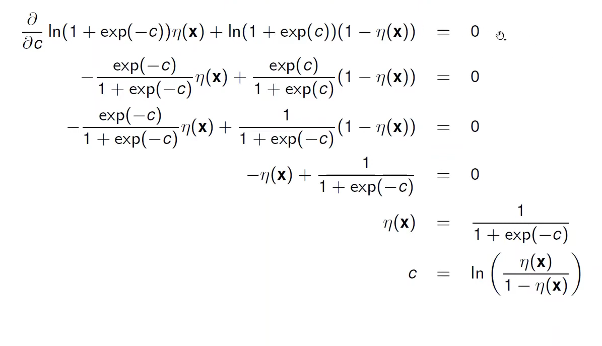
• Thus the risk minimiser is given by:

  \[f^*(x) = \ln(\frac{P(y \mid x)}{1 - P(y \mid x)})\]

  This function is undefined when $P(y \mid x) = 0/1$ but predicts a smooth curve which grows when $P(y \mid x)$ increases and equals $0$ when $P(y \mid x) = 0.5$.

---

§11.08: Deep Dive into Logistic Regression

https://github.com/slds-lmu/lecture_sl/raw/main/slides-pdf/slides-advriskmin-logreg-deepdive.pdf

---

§11.09: Brier Score

The brier score can be thought of as $L_2$ loss on probabilities $\pi(x)$ i.e.

\[L(y, \pi(x)) = (y - \pi(x))^2\]

The risk minimiser of the binary Brier Score is given by:

\[\pi^*(x) = P(Y=1|X=x)\]

---

§11.12: MLE vs ERM 1

• Consider regression from a MLE perspective: $y \mid x \sim p(y \mid x, \theta)$ where $y = f_{true}(x) + \epsilon$ and $f_{true}$ has params $\theta$ and $\epsilon$ is a R.V. that follows some distribution with $E[\epsilon] = 0$ (unbiased). Also, assume $\epsilon$ is independent from $x$ (no correlation/stochastic dependency).

• Then, given iid data $D = {(x^{(i)}, y^{(i)}) }_{i=1}^{n}$, in MLE we:

  \[\max_\theta L(\theta) = \Pi_{i=1}^{n} p(y^{(i)} | x^{(i)}, \theta)\] \[\Leftrightarrow\]

\[\min_\theta -l(\theta) = -\Sigma_{i=1}^n \log(p(y^{(i)} | x^{(i)}, \theta))\]

• From an ML perspective, we assume our hypothesis space corresponds to the space of parametrized $f_{true}$.

• Simply defining the negative log-likelihood as our loss function:

  \[L(y, f(x|\theta)) = -\log p(y|x, \theta)\]

• Then we get ERM, $R_{emp}(\theta) =$

  \[\Sigma_{i=1}^n L(y^{(i)}, f(x^{(i)}|\theta))\]

  which is equal to our MLE.

During comparisons we can ignore constants and use proportional equivalence as the constants don’t change the estimator.

• For every distribution $P_\epsilon$ we can derive an equivalent loss function, which leads to the same point estimator for the parameter vector $\theta$ as MLE. For example we can show that ERM with $L_2$ loss is equivalent to MLE with Gaussian errors.

💡 The other way does not necessarily hold. Given a loss function, we CAN NOT always get a probability distribution that yields equivalent MLE. Hinge loss is a one prominent example.

• The reverse direction holds If we can write the loss as $L(y, f(x)) = L(y - f(x)) = L(r)$ i.e. the loss function is a function of the residuals, then minimizing $L(y - f(x))$ is equivalent to maximizing $\log(p(y-f(x

  \theta))$ if

  1. $\log(p(r)) = a -bL(r)$ (affine transformation with $b >0)$ and
  2. $p$ is a pdf.

💡 Thus, a loss $L$ corresponds to MLE under some distribution if $\exists a \in \mathbb{R}, b> 0$ s.t $$ \int_{\mathbb{R}} e^{a - bL(r)} dr = 1 $$

---

§11.13: MLE vs ERM 2

• Laplace Errors $\Leftrightarrow L_1$ Loss
• Bernoulli RV $\Leftrightarrow$ Bernoulli Loss

---

§11.14: Properties of Loss Functions

• Why should we care about the loss function? Because the choice of the loss function implies certain statistical assumptions of the underlying distribution. Moreover some are more robust to outliers, and some have very high computational complexity.
• Robustness: A model is less influenced by outliers than by “in-liers” if the loss is robust. For example, outliers strongly influence the L2 loss.
• Smoothness: A property measured by the number of continuous derivatives. Derivative based optimisation require certain degrees of smoothness.
• Convexity: Convexity of the risk depends on both the loss function and $f(x \mid \theta)$.
• Convergence: Logistic Regression for example can never converge if data is linearly separable

---

§11.15: Bias-Variance Decomposition

• The generalisation error can be decomposed into three parts - bias, variance, and inherent noise. The expected error of learning algorithm $I_L$ for an induced model $\hat{f}_{D_n}$, on training sets of size $n$ when applied to fresh unseen observation is:

  \[GE_n(I_L) = E_{D_n \sim P^n_{xy}, (x,y) \sim P_{xy}} [L(y, \hat{f}_{D_n}(x)]\]

  i.e. we need to take an expectation over all training sets of size n as well as the independent test observation.

• The GE can be decomposed into the following three components:
  1. Irreducible Noise: $\sigma^2$
  2. Variance: $\operatorname{Var}{D_n} (\hat{f}{D_n}(x) \mid x, y)$ expresses on average how much $\hat{f}_{D_n}$ fluctuates around test points if we vary the training data. It expresses the learner’s tendency to overfit.
  3. Bias: $E_{xy}[(f_{\text{true}}(x) - E_{D_n}[\hat{f}_{D_n}(x)])^2 \mid x, y]$ expresses how much on average we are off at test locations i.e. underfitting. Models with high capacity typically have low bias.
• The performance of a model depends on its ability to fit the data well and generalise unseen data.

---

§11.16: Bias-Variance Decomposition Deep Dive

https://github.com/slds-lmu/lecture_sl/raw/main/slides-pdf/slides-advriskmin-bias-variance-decomposition-deepdive.pdf