Chapter 16: Linear Support Vector Machine
This chapter introduces the linear support vector machine (SVM), a linear classifier that finds decision boundaries by maximizing margins to the closest data points, possibly allowing for violations to a certain extent.
§16.01: Linear Hard Margin SVM (Primal)
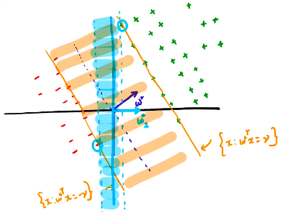
- We know that the number of mistakes committed/iterations required by the perceptron learning algorithm is bounded by $\frac{R^2}{\gamma^2}$ where $R$ is the radius of the ball inside which the farthest datapoint lies at and $\gamma$ is the margin from origin to the nearest datapoint.
- Given these separators $w^\ast$ and $w_2^\ast$, which one would be better? Intuitively it feels like $w^\ast$ would be better since it classifies with higher margin. This is also evident from the above mentioned bound. The higher the $\gamma$, lower the bound which is good. However there is nothing in the perceptron learning algorithm that ensures that $w^\ast$ is found. It could output $w_2^\ast$. We need to formulate the optimisation problem differently
-
So we can start with a formulation as follows:
\[\begin{align*} \max_{\theta, \theta_0} \quad & \gamma \\ \text{s.t.} \quad & y^{(i)}(\theta^T x^{(i)} + \theta_0) \geq \gamma \end{align*}\]Now this is a good place to start, but there is a problem with this. Given a $\theta$ and $\theta_0$, we can just multiply it by a constant $c$ such that the new margin now is $c*\gamma$. This means this maximisation problem has no upper limit and thus has no solution.
-
Since it is primarily the direction where the margin is the highest is what we are looking for, we can only consider $\theta$ which has norm 1:
\[\begin{align*} \max_{\theta, \theta_0} \quad & \gamma \\ \text{s.t.} \quad & y^{(i)}(\theta^T x^{(i)} + \theta_0) \geq \gamma \\ & \mid \mid \theta \mid \mid^2 = 1 \end{align*}\] -
Since the dataset $x^{(i)}$ are fixed, and once we fix the $\theta$, the $\gamma$ gets fixed i.e. the $\gamma$ is a function of $\theta$, what we can do instead is to fix the $\gamma$ and maximise the width between the two hyperplanes instead. It can be shown that the $\text{width}(\theta) = \frac{2}{||\theta||^2}$. Thus our problem now is:
-
This formulation is a convex optimisation problem with quadratic objective and linear constraints is now equivalent to:
\[\begin{align*} \min_{\theta, \theta_0} \quad & \frac{1}{2}||\theta||^2 \\ \text{s.t.} \quad & 1 - y^{(i)}(\theta^T x^{(i)} + \theta_0) \leq 0 \end{align*}\] -
Note that there exist instances of $(x^{(i)}, y^{(i)})$ where the constraints hold with equality. These are called the support vectors as they lie at a distance of $\gamma = \frac{1}{\mid \mid \theta \mid \mid^2}$ from the separating hyperplane. Note that we could delete all the points that aren’t support vectors and we would still arrive at the same solution.
§16.02: Linear Hard Margin SVM (Dual)
-
Solving such a constrained optimisation problem is usually done using Lagrange Multipliers. The problem is thus transformed into the following:
\[\min_{\theta, \theta_0} \max_{\alpha \geq 0} \frac{1}{2} ||\theta||^2 + \Sigma_{i=1}^n \alpha_i(1-\theta^T x^{(i)} + \theta_0)y^{(i)}\] -
Since both the constraints and the objective were convex, the $\min \max$ has a convex objective and we can hence switch the order to $\max_{\alpha \geq 0} \min_{\theta,\theta_0}$. Now what this allows us to do is that for some $\alpha \geq 0$, we can now solve the inner $\min_{\theta, \theta_0}$ as an unconstrained optimisation problem:
\[\min_{\theta, \theta_0} \frac{1}{2} ||\theta||^2 + \Sigma_{i=1}^n \alpha_i(1-\theta^T x^{(i)} + \theta_0)y^{(i)}\] -
At the optimum we have $\nabla_\theta = 0$:
\[\theta^*_{\alpha} - \Sigma_{i=1}^n \alpha_i x^{(i)} y^{(i)} = 0 \Leftrightarrow \theta^*_{\alpha} = \Sigma_{i=1}^n \alpha_i x^{(i)} y^{(i)}\]and $\nabla_{\theta_0} = 0$ gives us:
\[\Sigma_{i=1}^n \alpha_i y^{(i)} = 0\] -
Plugging these back into the objective function in place of $\theta$, we get:
\[\max_{\alpha \in R^n} \Sigma \alpha_i - \frac{1}{2} \Sigma \Sigma \alpha_i \alpha_j y^{(i)} y^{(j)} <x^{(i)}, x^{(j)}>\] \[\begin{align*} \equiv \max_\alpha \quad & 1^T \alpha - \frac{1}{2} \alpha^T \text{diag}(y) XX^T \text{diag}(y) \alpha \\ \text{s.t.} \quad & \alpha^T y = 0 \\ & \alpha \geq 0 \end{align*}\] -
Now if $(\theta, \theta_0, \alpha)$ fulfills KKT conditions, it solves both the primal and dual problem and we know that $\theta$ is simply a linear combination of our data points. The complementary slackness condition gives us that either $\alpha_i = 0$ or $(\theta^T x^{(i)} + \theta_0) y^{(i)} = 1$. This tells us that we solve the dual and we get $\alpha_i > 0$, then these points necessarily lie on the supporting hyperplane and is therefore a support vector.
§16.03: Linear Soft Margin SVM
-
The hard margin SVM only has a solution if the dataset is linearly separable. However that is not often the case and we may have some outliers. The idea is that we want a large margin for most samples, and allow some violations which are penalised. This can be done by modifying the constraint as follows:
\[y^{(i)}(\theta^T x^{(i)} + \theta_0) + \epsilon_i \geq 1\] - Previously the constraint forced the margin to be at least 1. Now, if the margin is not 1, then we allow them “to pay a bribe”. However this “bribe” needs to be penalised in the objective. Even for a linearly separable data, we could have a model with few violations but a high margin.
-
The linear soft-margin SVM is a convex quadratic program. Its primal is given by:
\[\begin{align*} \min_{\theta, \theta_0, \epsilon^{(i)}} \quad & \frac{1}{2} ||\theta||^2 + C \Sigma \epsilon^{(i)} \\ \text{s.t.} \quad & y^{(i)}(\theta^T x^{(i)} + \theta_0) \geq 1 - \epsilon^{(i)} \\ & \epsilon^{(i)} \geq 0 \end{align*}\]with $C > 0$ that controls how much we maximise the margin vs how much we minimise margin violations.
- $C=0 \Rightarrow$ there’s no penalty to violating the margins and hence $\theta = 0$ will be the optimal solution.
- $C = \infty \Rightarrow$ there’s an infinite penalty for violating the margins and hence this problem will have solution only if dataset is linearly separable.
-
We can now derive the dual for soft-margin SVM as well. Using the method of Lagrange, the problem is transformed into:
\[\min_{\theta, \theta_0, \epsilon^{(i)}} \max_{\alpha^{(i)},\mu^{(i)}} \frac{1}{2} ||\theta||^2 + C \Sigma_{i=1}^n \epsilon^{(i)} -\Sigma_{i=1}^n \alpha_i(y^{(i)} (\theta^T x^{(i)} + \theta_0) - 1 + \epsilon^{(i)}) - \Sigma_{i=1}^n \mu_i \epsilon^{(i)}\]Since it’s a quadratic programming problem (i.e. convex) we can switch the min and max. For a fixed $\alpha$ and $\mu$, we can then solve for $\theta^{\alpha, \mu}, \theta_0^{\alpha, \mu}, \epsilon^{\alpha, \mu}$ as an unconstrained optimisation problem. Solving for it, we get:
\[\theta^{\alpha, \mu} = \Sigma_{i=1}^n \alpha_i y^{(i)} x^{(i)}, \Sigma_{i=1}^{n} \alpha_i y^{(i)} = 0, \alpha_i + \mu_i = C\] - Plugging them in, we get the dual formulation:

Complementary Slackness Conditions
Let $(\theta^\ast, \theta_0^\ast, \epsilon^*)$ be the primal solutions and $(\alpha^\ast, \mu^\ast)$ be the dual solutions. Then at optimality, the following complementary slackness conditions hold:
- $\alpha_i^\ast(1-y^{(i)}(\theta^{*T}x^{(i)} + \theta_0) - \epsilon^{(i)\ast}) = 0$
- $\mu_i^\ast(\epsilon^{(i)\ast}) = 0$
Case 1: $\alpha_i^\ast = 0$
Then $\mu_i^\ast = C$. From CS 2 we get, $\epsilon^{(i)\ast} = 0$ i.e. these points don’t “pay a bribe”. Furthermore, from CS 1, $1-y^{(i)}(\theta^{\ast T}x^{(i)} + \theta_0) - \epsilon^{(i)\ast} \leq 0 \Rightarrow y^{(i)}(\theta^{\ast T}x^{(i)} + \theta_0) \geq 1$ i.e. these points are classified correctly. They either are on the supporting hyperplane or are classified correctly and are away from the supporting hyperplane.
Case 2: $\alpha_i^\ast \in (0, C)$
We get that $\mu_i^\ast > 0 \Rightarrow_{CS 2} \epsilon^{(i)\ast} = 0$ i.e. these points also don’t “pay a bribe”. Furthermore from CS 1 we get $1-y^{(i)}(\theta^{\ast T}x^{(i)} + \theta_0) = 0$ i.e. these points lie exactly on the supporting hyperplane.
Case 3: $\alpha_i^\ast = C$
From CS 1 we get that $1-y^{(i)}(\theta^{\ast T}x^{(i)} + \theta_0) + \epsilon^{(i)\ast} = 0 \Rightarrow \epsilon^{(i)\ast} = 1-y^{(i)}(\theta^{\ast T}x^{(i)} + \theta_0)$ i.e. these points “pay a bribe”. This implies that these points are either classified correctly with not enough margin or are classified incorrectly.
§16.04: SVMs and ERM
-
In the optimum, the inequalities will hold with equality as we minimise the “bribes”, so $\epsilon^{(i)} = 1 - y^{(i)} f(x^{(i)}) \geq 0$. Thus we can rewrite the objective function as follows:
\[\frac{1}{2} ||\theta||^2 + C \Sigma_{i=1}^n L(y^{(i)}, f(x^{(i)})) \text { where } L = \max(1 - yf, 0)\] - This is now simply Risk Minimisation with L2 Regularisation and this particular loss function is called the Hinge Loss. This above definition of the SVM problem does not require any geometrical interpretation, is convex, and without constraints. However it is non-differentiable due to the $\max$.
- We can also generalise the SVM by using other loss functions. One notable example is using the log-loss which is the same as Logistic Regression with $L2$ regularisation. However it is important to note that these other loss functions don’t generate sparse solution (i.e. the solution only being dependent on a few data points).
§16.05: SVM Training
- Until now we didn’t focus on the training. Should we solve the primal or the dual ? SVMs are usually trained in the dual however it can also be trained in the primal.
- The unconstrained variant of the SVM i.e. the one with hinge loss cannot be solved using gradient descent since the max function is non-differentiable $\Rightarrow$ Either use a differentiable loss like squared hinge (which results in non-sparsity of our solution) or use subgradient methods.