Chapter 18: Boosting

This chapter introduces boosting as a sequential ensemble method that creates powerful committees from different kinds of base learners."

§18.01: Introduction to Boosting / AdaBoost

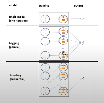
Bagging is Bootstrap Aggregating where you typically overfit learners from bootstrapped datasets (sampling with replacement) and aggregate across all the weak learners. So you typically start off with low bias, high variance learners (basically overfitted) and end up with a low bias, low variance bagged learner.
The basic premise of boosting is to to train weak (underfit) learners with high bias, low variance on weighted datasets sequentially. After each iteration, misclassified points are given a higher weight for the next iteration.

AdaBoost

We use binary classifiers as weak base learners from a hypothesis space $\mathcal{B}$, denoted by $b^{[m]} \text{ or } b(x, \theta^{[m]})$ which are hard-labelers and output ${-1,1}$. Decision score of the ensemble of size $M$ is then the weighted average :
\[f(x) = \Sigma_{m=1}^{M} \beta^{[m]} b(x, \theta^{[m]}) \in R\]
where $\beta^{[m]}$ is higher for base learners which have greater accuracy.

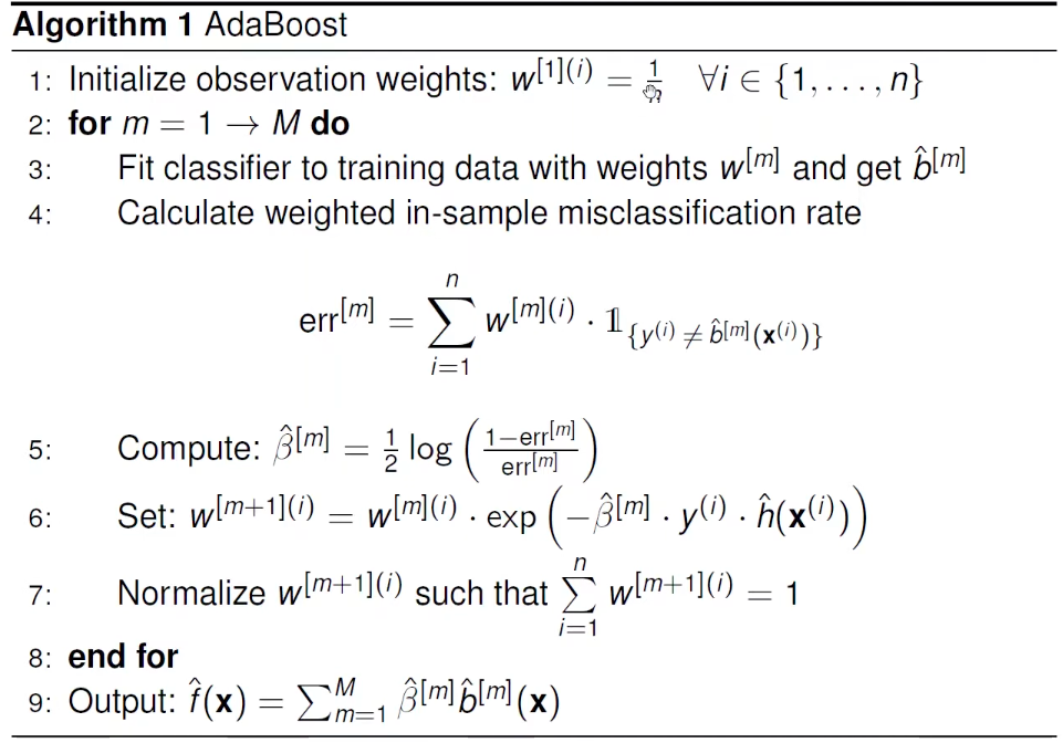
Adaboost tends to overfit for a large number of iterations whereas RFs don’t.

§18.02: Boosting Concept

We can now generalise AdaBoost as wanting to learn additive models where $f$ is an additive model of base learners $b$
\[R_{emp}(f) = \Sigma_{i=1}^n L(y^{(i)}, f(x^{(i)})) = \Sigma_{i=1}^n L(y^{(i)}, \Sigma_{m=1}^M \beta^{[m]} b(x, \theta^{[m]}))\]
Because of its additive structure, it is difficult to jointly minimise since it is a very high dimensional problem. If $\theta \in R^p$ , then we would need to jointly optimise for $p \times M$ parameters. To reduce the model complexity, we can iteratively do this where
\[(\hat{\beta}^{[m]}, \hat{\theta}^{[m]}) = \operatorname{argmin}_{\beta, \theta} \Sigma_{i=1}^{n} L(y^{(i)}, \hat{f}^{[m-1]}(x^{(i)}) + \beta b(x^{(i)}, \theta))\]
i.e. optimise in a greedy fashion where at each tilmestep we take the additive model thus far and optimise parameters for adding another base learner.
Gradient Boosting is a forward stagewise additive modelling method which is essentially “Gradient Descent in the function space”. At each time step, we optimise the parameters of a base learner such that it minimises the $L2$ loss wrt to the pseudo-residuals i.e.
1. Initialise $\hat{f}^{[0]}(x) = \operatorname{argmin}_\theta \Sigma_i L(y^{(i)}, b(x^{(i)}, \theta))$. Then for all $m: 1 \to M$
2. Calculate pseudo-residuals: $\tilde{r}^{[m](i)} = -[\frac{\partial L(y^{(i)}, f(x^{(i)}))}{\partial f(x^{(i)})}]_{f = \hat{f}^{[m-1]}}$
3. Fit a (regression) base learner s.t. $\hat{\theta}^{[m]} = \operatorname{argmin}_\theta \Sigma_i (\tilde{r}^{[m](i)} - b(x^{(i)}, \theta))^2$
4. \[\hat{f}^{[m]}(x) = \hat{f}^{[m-1]} (x) + \beta^{[m]} b(x, \hat{\theta}^{[m]})\]
where $\hat{\beta}^{[m]}$ could either be a small constant value or optimised for using exact linear search.
Boosting with linear model as base learner converges pretty much in 1 iteration as it is simply the same as LR with $L2$ Loss.

§18.03: Boosting Illustration

§18.04: Boosting Regularization

Since GB can easily overfit, it is important to regularise it. Three main options for regularisation:

Limit number of iterations M
Limit depth of trees
Use small learning rate $\alpha$

§18.05: Boosting for Classification

We can also apply the same principles for a binary classification task for example in a logistic regression with Bernoulli loss:
\[L(y, f(x)) = -y f(x) + \log(1 + e^{f(x)})\]
Then, the pseudo-residuals $\tilde{r}(f) = y - s(f(x)) = y - \pi(f(x))$ i.e. $0-1$ label minus the predicted probability. The rest works the same as before. Note that we still fit the base learners using the $L2$ loss against the Pseudoresiduals.
We can also use the exponential loss and it can be shown that it is equivalent to AdaBoost.
In the multi-class scenario we have $g$ discriminant functions (one for each class) with each being an additive model. We can use the multinomial log-loss (cross-entropy):
\[L(y, f_1(x),...,f_g(x)) = -\Sigma_k 1_{\{y=k\}} \ln \pi_k(x)\]
where $\pi_k$ is the Softmax function. In this case the pseudo-residuals are $1_{{y=k}} - \pi_k(x)$.
The rest of the procedure in multi-class case is the same. Do note that each boosting iteration will fit $g$ additive models.

§18.06: Gradient Boosting with Trees 1

Trees are very popular base learners for Gradient Boosting as they have no problems with categorical variables, outliers, missing values, monotonic transformations of features. Furthermore they can be fitted quickly and have a simple built-in variable selection.

The depth of the tree in our base learner has a huge impact on the interaction effect between features since trees themselves can be written as weighted additive models to the leaf node: $b_(x) = \Sigma_t c_t 1_{{x \in R_t}}$.

A tree of depth=1 is simply a decision stump and the decision is split across just one feature:	In a tree of depth=2, we have two-way interaction between features: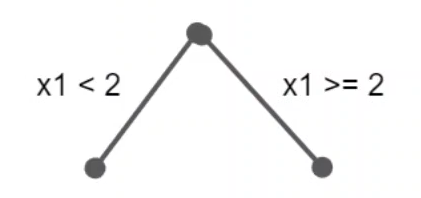

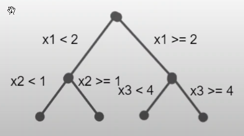
Thus an additive GB with decision stumps as base learners could be refactored as: $$ f(x) = f_0 + \sum_{j=1}^p f_j(x_j) $$	Thus an additive GB with tree depth=2 as base learners could be refactored as: $$ f(x) = f_0 + \sum_{j=1}^p f_j(x_j) + \sum_{j \ne k} f_{j,k}(x_j, x_k) $$

When we only use decision stumps, there is no interaction effect between features. The marginal effects add up to joint effects. When using trees of depth 2, the marginal effects do NOT add up to joint effect as the interaction term is still needed.

§18.07: Gradient Boosting with Trees 2

The Gradient Boosted model is still additive:
\[f^{[m]}(x) = f^{[m-1]}(x) + \alpha^{[m]}b^{[m]}(x) = f^{[m-1]}(x) + \Sigma_t \tilde{c}_t^{[m]}1_{\{x \in R_t\}}\]
where $\tilde{c}_t = \alpha^{[m]} c_t^{[m]}$. After the tree (base learner) has been fitted against the pseudo-residuals, we can adapt the tree individually and directly loss optimally:
\[\tilde{c}_t^{[m]} = \operatorname{argmin}_c \Sigma_{x^{(i)} \in R_t^{[m]}} L(y^{(i)}, f^{[m-1]}(x^{(i)}) + c)\]

§18.08: XGBoost

\[R_{reg}^{[m]} = \Sigma_{i=1}^n L(y^{(i)}, f^{[m-1]}(x^{(i)})+b^{[m]}(x^{(i)})) + \lambda_1 J_1(b^{[m]}) + \lambda_2 J_2 (b^{[m]}) + \lambda_3 J_3(b^{[m]})\]

where $J_1 = T^{[m]}$ : Number of leaves to peanlise tree depth, $J_2 = \mid \mid c^{[m]} \mid \mid_2^2$: $L2$ penalty over leaf values and $J_3 = \mid \mid c^{[m]}\mid \mid_1$: $L1$ penalty over leaf values.

XGB uses both data subsampling and feature subsampling (like Random Forests). Each tree is grown till max-depth and then pruned.
DART introduces the idea of dropout regularisation used in DL. In each iteration, when learning a new base learner we fit the base learner against the pseudo-residuals of $\hat{f}^{[m-1]}$ which is an additive model of base learners. Instead of using all the base learners, only a subset $D$ is used where each base learner is dropped with a probability $p_{drop}$.
When trees are dropped, the current ensemble’s prediction is artificially lower (or higher) than it would be if all trees were active. Imagine you have an ensemble whose full prediction (with all trees) for a particular instance is 10. Now consider a training iteration where a couple of trees—each contributing 1 unit—are dropped. With these trees missing, the effective ensemble prediction is 10 − 2 = 8. This is called overshot predictions. Therefore we scale the base learners in the following way:
1. $\frac{1}{1+\mid D \mid} \hat{b}^{[m]}$
2. $\frac{ \mid D \mid}{\mid D \mid+1} \hat{b} \text{ } \forall b \in D$
$p_{drop}=0:$ Ordinary Gradient Boosing and $p_{drop}=1:$ all base learners are trained independently and equally weighted. This is similar to Random Forests. Hence, $p_{drop}$ gives us a smooth transition from Gradient Boosting to Random Forests.

§18.09: Component Wise Boosting Basics 1

In Component-Wise Boosting, we have $J$ classes of base learners, with each class associated with one feature. The gradient boosting procedure follows the standard approach but includes these additional steps in each iteration:
1. for $j: 1 \to J$: Fit regression base learner $b_j \in \mathcal{B}_j$ to the vector of pseudo-residuals as follows:
  \[\hat{\theta}_j^{[m]} = \operatorname{argmin}_{\theta \in \Theta_j} \Sigma_i (\tilde{r}^{[m]} - b_j(x^{(i)}, \theta))^2\]
2. Choose base learner from $J$ base learners that minimize the L2 loss:
  \[j^{[m]} = \operatorname{argmin}_j \Sigma_i (\tilde{r}^{[m]} - b_j(x^{(i)}, \theta))^2\]
In each iteration, only one feature is selected. Since these base learners are additive, we can combine the parameters at the end of our GB procedure to get one parameter per feature, making the model highly interpretable.
A learning rate dampens the effect of the added model. As a result, the same feature and its base learner are often selected repeatedly for several iterations before moving to the next. This means the final model typically uses fewer than $\leq M$ features.
The selection of just one feature per iteration creates a natural feature selection mechanism within the algorithm.

§18.10: Component Wise Boosting Basics 2

For categorical variables, we can either have one base learner that simultaneously estimates all categories or we could have a binary base learner per category. Advantages of using a single base learner is a faster estimation (especially if there are a lot of categories). Penalisation and selection becomes difficult with binary learners as they have exactly one degree of freedom.
There are two ways we can handle the intercept parameter. We can add a base learner for the intercept and remove all the intercepts from other base learners (this assumes that all covariates are centered). Or we could include an intercept in each base learner and aggregate it into a global intercept.

§18.11: CWB and GLMs

In the simplest case when we use $b_j(x_j, \theta) = \theta x_j$ as our base learners, in the limit this will converge to the MLE solution. Usually boosting model is not run until convergence. Early stopping is often used for regularisation and feature selection.
By specifying the loss as Negative Log Likelihood of exponential family with an appropriate link function, CWB is equivalent to GLM.
When we don’t use an exponential family of distribution, the resulting model may look like GLM. However we don’t have valid standard errors and thus cannot provide confidence intervals.

§18.12: Advanced CWB

We can also use non-linear base learners like P- or B- splines which make the model equivalent to Generalised Additive Model (GAM).
Nonlinear Effect Decomposition: If the possible choices for base learners include both linear and non-linear learners, then the algorithm will almost always choose the non-linear one since it is more flexible. Therefore there is a decomposition available where we break it down to constant, linear effect, and the difference between non-linear and linear effect. This ensures that linear effects are also learned. **There are also regularisation methods to make the degrees of freedom equal through penalisation.
If we use single features in base learners, we consider each BL as a wrapper around a feature. Since they are additive, we can get the final effect of a feature on the target. Hence $\hat{f}$ can be decomposed into marginal feature effects (partial dependence plots) PDPs.
Feature Importance: We can exploit the additive structure of the boosted ensemble to compute measure of variable importance. One simple measure for feature $j$ is to go over all iterations where $b_j$ was selected and sum up the reduction in empirical risk:
\[VI_j = \Sigma_{m=1}^{m_{stop}}(R_{emp}(f^{[m-1]}(x)) - R_{emp}(f^{[m]}(x))) 1_{j \in j^{m}}\]