Chapter 2: Finite Markov Decision Processes

This chapter explores the fundamental concepts of Markov Decision Processes (MDPs) covering the agent-environment interface, goals and rewards, returns and episodes, and policies and value functions.

§2.01: The Agent-Environment Interface (Full RL Problem)

MDPs are a classical formalization of sequential decision making, where actions influence not just immediate rewards, but also subsequent situations, or states, and through those future rewards. Thus MDPs involve delayed reward and the need to trade off immediate and delayed reward.

MDPs are meant to be a straightforward framing of the problem of learning from interaction to achieve a goal. The learner and decision maker is called the agent. The thing it interacts with, comprising everything outside the agent, is called the environment. These interact continually, the agent selecting actions and the environment responding to these actions and presenting new situations to the agent. The environment also gives rise to rewards, special numerical values that the agent seeks to maximize over time through its choice of actions.

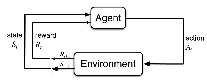
More specifically, the agent and environment interact at each of a sequence of discrete time steps, $t=0,1,…$ . At each time step $t$, the agent receives some representation of the environment’s state, $S_t$, and on that basis selects an action, $A_t$. One time step later, in part as a consequence of its action, the agent receives a numerical reward, $R_{t+1}$, and finds itself in a new state, $S_{t+1}$ The MDP and agent together thereby give rise to a sequence or trajectory that begins like this:

\[S_0, A_0, R_1, S_1, A_1, R_2, S_2,A_2, R_3,...\]

We use $R_{t+1}$ instead of $R_t$ to denote the reward due to $A_t$ because it emphasizes that the next reward and next state, $R_{t+1}$ and $S_{t+1}$, are jointly determined.

For finite MDP’s with finite states actions and rewards, we have a well defined discrete probability distribution $p$ that defines the dynamics of the MDP.

\[p(s', r | s, a) = \text{Pr}\{S_t = s', R_t=r | S_{t-1}=s, A_{t-1}=a\}\]

💡 A Markov decision process completely characterises the environment’s dynamics by $p$ i.e. The probability of each possible value of $S_t, R_t$ depends on the immediately preceeding states and actions $S_{t-1}, A_{t-1}$ alone.

---

§2.02: Goals and Rewards

The agent’s goal is to maximise the total amount of reward it receives. This means maximising not immediate reward, but cumulative reward in the long run. If we want it to do something for us, we must provide rewards to it in such a way that in maximising them the agent will also achieve our goals. It is thus critical that the rewards we set up truly indicate what we want accomplished. In particular, the reward signal is not the place to impart to the agent prior knowledge about how to achieve what we want it to do. Better places for imparting this kind of prior knowledge are the initial policy or initial value function.

💡 The reward signal is your way of communicating to the agent what you want achieved, not how you want it achieved.

---

§2.03: Returns and Episodes

• Episodic Tasks: In general we seek to maximise expected return. In the simplest case, the return is the sum of rewards where $T$ is a finite time-step:

  \[G_t = R_{t+1} + R_{t+2} + ... + R_{T}\]

  This approach makes sense where there is a notion of final time step and the agent-environment interaction breaks down to subsequences called episodes.

• Continuing Tasks: On the other hand, when the agent-environment interaction does not break down into identifiable episodes, but instead goes on continually without limit, we choose $A_t$ that maximises the expected discounted return:

  \[G_t = R_{t+1} + \gamma R_{t+2} + \gamma^2 R_{t+3} + ... = \Sigma_{k=0}^\infty \gamma^k R_{t+k+1}\]

• Unified Notation for Episodic and Continuing Tasks:

  • For episodic tasks we never have to distinguish between episodes. We are almost always considering a particular episode, or stating something that is true for all episodes.
  • We can modify the episodic task by considering episode termination to be entering a special absorbing state that transitions only to itself and generates only rewards of zero.
  • Thus the unified notation for episodic and continuing tasks including the possibility of $T=\infty, \gamma =1$ (but not both) is given by: \(G_t = \Sigma_{k=t+1}^T \gamma^{k-t-1}R_k\)

---

§2.04: Policies and Value Functions

A policy is a mapping from states to probabilities of selecting each possible action.

The value function of a state s under policy $\pi$, denoted $v_{\pi}(s)$ is the expected return when starting in s and following $\pi$ thereafter called the state-value function.

\[v_{\pi}(s) = \text{E}_{\pi}[ G_t | S_t=s] = \text{E}_{\pi}[ \Sigma_{k=0}^{\infty} \gamma^k R_{t+k+1}|S_t =s]\]

where $E_\pi$ denotes the expected value of a random variable given that the agent follows policy $\pi$. Note that, $v_{\pi}(s) = \Sigma_{a} \pi(a \mid s) q_{\pi}(s,a)$

The value of taking an action a in the state s under policy $\pi$, denoted by $q_{\pi}(s,a)$ as the expected return starting from s taking an action a and thereafter following policy $\pi$ is called as action-value function given by:

\[q_{\pi}(s,a) = \text{E}_{\pi}[G_t | S_t=s, A_t=a] = \text{E}_{\pi}[\Sigma_{k=0}^{\infty}\gamma^k R_{t+k+1} | S_t=s, A_t =a]\]

Also note that,

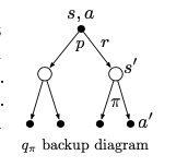
\[q_{\pi}(s,a) = \text{E}_{\pi}[G_t | S_t=s, A_t=a]\] \[=E_{\pi}[R_{t+1} + \gamma G_{t+1} | S_t=s, A_t =a] = \Sigma_{s',r} p(s',r | s,a)[r+\gamma v_{\pi}(s')]\]

Bellman Equation:

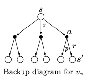
\[v_{\pi}(s) = \text{E}_{\pi}[ G_t | S_t=s] = \text{E}_{\pi}[R_{t+1} + \gamma G_{t+1} | S_t=s]\] \[= \Sigma_a \pi(a|s) \Sigma_{s', r} p(s', r | s, a) [r + \gamma \text{E}_\pi [G_{t+1} | S_{t+1} = s']]\] \[= \Sigma_a \pi(a|s) \Sigma_{s', r}p(s',r|s,a)[r + \gamma v_\pi(s')]\]

When something is conditioned on $s$ alone, think of this backup diagram. You’ll have to sum over $\pi(a \mid s)$ incase you are using the four-argument $p(s', r \mid s,a)$	When something is conditioned on $s,a$, think of this backup diagram. Since you already know s,a you can directly use the four-argument $p(s', r \mid s, a)$

---

§2.05: Optimal Policies

A policy $\pi$ is defined to be better than or equal to a policy $\pi’$ if its expected return is greater than or equal to that of $\pi’$ for all states. In other words, $\pi \geq \pi’$ if and only if $v_\pi(s) \geq v_{\pi’}(s) \forall s$.

\[v_*(s) = \max_\pi v_{\pi}(s)\]

Optimal policies also share the same optimal action-value function:

\[q_*(s,a) = \max_{\pi} q_\pi(s,a)\]

For the state-action pair (s,a), this function gives the expected return for taking action a in state s and thereafter following an optimal policy. Thus we can write

\[q_*(s,a) = E[R_{t+1} + \gamma v_*(S_{t+1}) | S_t = s, A_t = a]\]

Under Bellman Optimality, (by definition) the value of a state under an optimal policy must be equal to the expected return for the best action from the state:

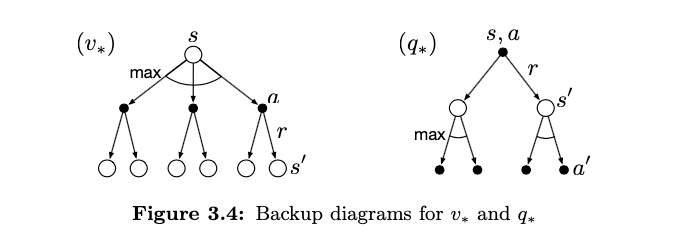
\[\begin{align*} v_*(s) &= \max_a q_{\pi_*}(s,a) \\ &= \max_a \mathbb{E}_{\pi_*}[G_t \mid S_t = s, A_t = a] \\ &= \max_a \mathbb{E}_{\pi_*}[R_{t+1} + \gamma G_{t+1} \mid S_t = s, A_t = a] \\ &= \max_a \mathbb{E}[R_{t+1} + \gamma v_*(S_{t+1}) \mid S_t = s, A_t = a] \\ &= \max_a \sum_{s', r} p(s', r \mid s, a)\left[r + \gamma v_*(s')\right] \end{align*}\]

Similarly under Bellman Optimality,

\[q_*(s,a) = E[R_{t+1} + \gamma \max_{a'}q_*(S_{t+1}, a') | S_t = s, A_t = a] \\ = \Sigma_{s', r} p(s', r | s, a) [r + \gamma \max_{a'}q_*(s',a')]\]

For finite MDP’s the above equations have a unique solution. It is a system of equations, one for each state so for n states there n equations and n unknowns. The beauty of bellman optimality is that if one uses $v_*$ to evaluate short term consequences i.e. use it as a greedy policy, then it is also optimal in the long term.

§2.06: Policy Evaluation

Consider a sequence of approximate value functions $v_0, v_1, …$ each mapping $s$ to $R$ (the real numbers). The initial approximation, $v_0$, is chosen arbitrarily (except that the terminal state, if any, must be given value 0), and each successive approximation is obtained by using the Bellman equation for $v_\pi$ as an update rule:

\[v_{k+1}(s) = E_\pi[R_{t+1} + \gamma v_k(S_{t+1}) | S_t = s] \\ = \Sigma_a \pi(a|s) \Sigma_{s', r} p(s',r|s,a)[r + \gamma v_k(s')]\]

The sequence ${v_k}$ in general converges to $v_\pi$ as $k \to \infty$. This is called iterative policy evaluation. Each iteration updates the value of every state once to produce the new approximate value function $v_{k+1}$. All the updates done in DP are called expected updates because they are based on an expectation over all possible next states rather than a sample next state.