Chapter 2: Interpretable Models

Some machine learning models are already inherently interpretable, e.g. simple LMs, GLMs, GAMs and rule-based models. These models are briefly summarized and their interpretation clarified.

§2.01: Inherently Interpretable Models - Motivation

• The most straightforward approach to achieving interpretability is to use inherently interpretable models. There are certain classes of models that are deemed inherently interpretable like linear models, additive models, decision trees, rule-based learning, model/component-based boosting, etc.

  • Pros: For such cases, model-agnostic methods are often not required and this eliminates a source of error. Furthermore they are often simple and require fairly small training time. Some classes like GLMs can estimate monotonic effects. Since many people from different domains are familiar with interpretable models, it increases trust and facilitates easier communication of results.

  • Cons: These models often require strong assumptions about the data (normal errors for LRs or assuming linear structure when the underlying data is quadratic). When these assumptions are wrong models may perform poorly. Inherently interpretable models may also be hard to interpret e.g. a linear model with a lot of features and interactions or a decision tree with a huge depth. Furthermore due to their limited flexibility they may struggle to model complex relationships.

• An important thing to remember is that inherently interpretable models do not provide all types of explanations. For example counterfactual explanations are useful for even LRs and decision trees.

• Whilst some argue that interpretable models should be preferred to models that require post-hoc analysis, they sometimes require a lot of time and energy on data pre-processing and/or manual feature engineering. It is also hard to achieve this for data where end-to-end learning is crucial i.e. feature extraction for image/text/audio data often leads to information loss leading to bad performance.

---

§2.02: Linear Regression Model (LM)

• The Linear Regression Model is given by:

  \[y = \theta_0 + \theta_1 x_1 + ... + \theta_p x_p + \epsilon = x^T \theta + \epsilon\]

  where the model consists of $p+1$ weights due to the intercept $\theta_0$

Assumptions of the Linear Model

1. Linear Relationship between the features and target.
2. $\epsilon$ and $y \mid x$ are normally distributed with homoscedastic (constant) variance i.e. $ \epsilon \sim N(0, \sigma^2) \Rightarrow y \mid x \sim N(x^T \theta, \sigma^2)$. If the homoscedastic variance assumption is violated then inference based metrics like $p-$value or $t-$ statistics are no longer valid/reliable.
3. Features $x_j$ are independent from the error term $\epsilon$. Therefore if we plot a single feature against the error term, we should see a point-cloud with no trend.
4. No or little multicollinearity i.e. there are no strong correlations in our dataset.

Interpretation of Weights (Feature Effects)

• Numerical $x_i$: Increasing $x_i$ by one unit changes the outcome $y$ by $\theta_i$ units ceteris paribus (cp).
• Binary $x_j$: When the binary feature $x_j$ is active (i.e. 1), then the outcome $y$ changes by $\theta_j$ units compared to the reference category being that the feature is inactive i.e. $x_j = 0$ cp.
• Categorical Feature $x_k$ with $L$ categories: We create $L-1$ one-hot encoded binary features $(x_{k,1},…x_{k,L-1})$ each having its own weight. The left out category is our reference category. The interpretation now follows the same as for binary features. If we move from the reference category to a different category then the change in the outcome is weight of the category.

Inference

• The feature importance is given by the $t-$statistic value:

  \[| t_{\hat{\theta_j}} | = | \frac{\hat{\theta_j}}{SE(\hat{\theta_j})}|\]

  where high $t-$ values indicate important (significant) features.

• The probability of obtaining a more extreme test statistic assuming $H_0: \theta_j = 0$ i.e. assuming feature $j$ is “useless” (not significant) is given by the $p-$value. A high $\mid t \mid$ corresponds to a small $p-$value.

---

§2.03: LM - Interactions and LASSO

• The standard linear regression can be extended by including higher order effects $(x_j^2)$ or interaction effects $(x_i * x_j)$ which have their own weights. Both of these effects make the model more flexible but also make it less interpretable. Unlike ML model (like NN for eg), we need to perform feature engineering and specify all effects we want to model. Now the marginal effect can no longer be interpreted by single weights anymore.

  

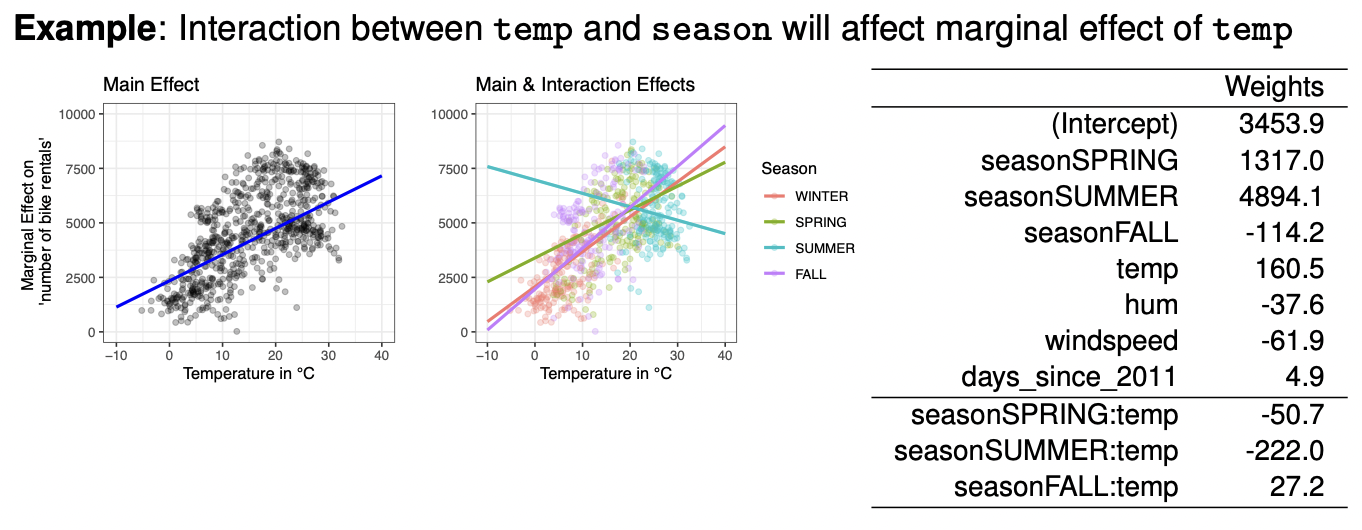
• With the reference season category being winter, here’s how we interpret interaction effects, an increase in the temperature by $1$ degree:
  1. In winter, the number of bike rentals change by $160.5$.
  2. In spring, the number of bike rentals change by $160.5 - 50.7 = 109.8$.
  3. In summer, the number of bike rentals change by $160.5 - 222.0 = -61.5$ (decrease).
  4. In fall, the number of bike rentals change by $160.5 + 27.2 = 187.7$.

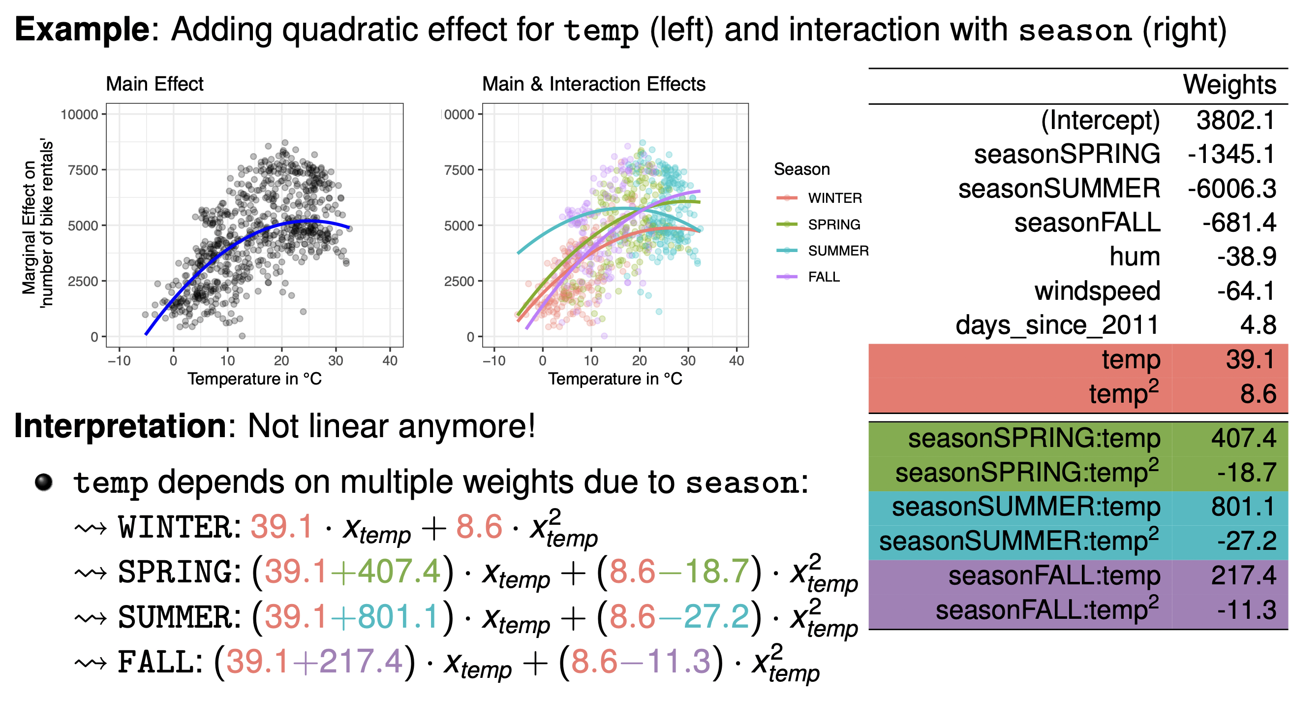
• Adding a quadratic effect for temperature for example makes our interpretation non-linear and the effect of temperature on bike-rentals is now determined by two coefficients:

  \[\theta_{temp} x_{temp} + \theta_{temp^2} x_{temp^2}\]

• Adding in quadratic and interaction effects makes the problem even more complicated to interpret:

  

Regularization via LASSO

• LASSO adds an $L_1-$norm penalization term to the least squares optimization problem. This shrinks some feature weights to 0 resulting in a sparser and more interpretable models. Here the penalization parameter $\lambda$ must be chosen using cross-validation.

💡 For one-hot encoded categorical variables i.e. $L$ categories resulting in $L-1$ binary variables, LASSO sees each binary variable as a separate variable and therefore only some of the categorical variables could get shrunk to 0. If we instead want either all or none of the $L-1$ binary variables to be shrunk then we could use Group LASSO.

---

§2.04: Generalized Linear Models

• The problem with LM and the variations with higher order and interaction effects we saw previously is that the assumption of $y \mid x \sim N(x^T \theta, \Sigma^2)$ does not always hold. If the target/outcome is a binary variable then a Bernoulli/Binomial distribution might be more apt. Similar for count variables, the poisson might work better. For time until first event, a gamma distribution would be suitable.

• GLMs extend LMs by still using a linear score, but allowing for distributions from the exponential family where a link function $g$ links the linear score/predictor $x^T \theta$ to the expectation of the conditional distribution i.e. :

  \[g(E(y | x)) = x^T \theta \Leftrightarrow E(y|x) = g^{-1}(x^T \theta)\]

  For LM, the $g$ is simply the identity function.

• The link function $g$, interaction and higher order effects need to be manually specified. The interpretation of the feature effects is therefore determined by the link function.

Logistic Regression

• The logistic regression is equivalent to the GLM with bernoulli distributed conditional expectation and the logit/sigmoid link function.

  \[g(x) = \log(\frac{x}{1 - x}) \Rightarrow g^{-1}(x) = \frac{1}{1 + e^{-x}}\]

• The logistic regression models the probabilities for binary classification through:

  \[\pi(x) = E(y | x) = P(y=1| x) = g^{-1}(x^T \theta) = \frac{1}{1 + e^{-x^T \theta}}\]

• If we rearrange the terms to solve for $x^T \theta$, you will see that the log-odds is linear i.e.

  \[\log(\frac{\pi(x)}{1-\pi(x)}) = x^T \theta\]

• This means that changing $x_j$ by one unit, changes the log-odds of class 1 compared to class 0 by $\theta_j$. However interpreting wrt to the odds-ratio is more common because the odds-ration is given by $\frac{\pi(x)}{1-\pi(x)} = e^{x^T \theta}$. Now if we compare the odds when $x_j$ increments by 1 against $x_j$, the ratio:

  \[\frac{odds_{x_j + 1}}{odds} = \frac{e^{\theta_0 + ... + \theta_j (x_j + 1) + ...}}{e^{\theta_0 + ... + \theta_j x_j + ...}}= e^{\theta_j}\]

  Thus, changing $x_j$ by 1 unit, changes the odds-ratio by a (multiplicative) factor of $e^{\theta_j}$.

• Note how logistic regression will always give rise to a linear classifier. The decision boundary will always be a $p-$dimensional hyperplane. This is because a threshold $t$ is set such that it is classified as 1 if $\pi(x) > t$ and classified as 0 otherwise.

  • For $t=0.5$: $x^T \theta = 0$ as log-odds is 0 at 0.5. This is a $p-$dimensional hyperplane.
  • For $t \neq 0.5$: $x^T \theta = \log(\frac{t}{1-t})$ which is also a $p-$dimensional hyperplane with the intercept being shifted.

💡 Changing the threshold does not change the linearity, only the location

---

§2.05: Rule-based Models

Decision Trees

• The main idea of decision trees is to partition data into subsets based on cut-off values in features (found by minimizing split criterion via greedy search especially in CART algorithms) and predict constant mean $c_m$ in leaf node $R_m$:

  \[\hat{f}(x) = \Sigma_{m=1}^M c_m 1\{ x \in R_m \}\]
• The structure of a (shallow) decision tree is nicely interpretable. They can be applied to both regression and classification problems and are able to model interactions and “non-linear” effects (basically a curve gets modeled like a Riemann sum by splitting across features). Furthermore it is able to handle mixed feature spaces and missing values as each rule is for a specific feature-value pair.
• We can simply interpret a decision tree by following its path to the leaf node. Decisions trees are also able to give us a feature importance measure by aggregating improvement in split criterion over all splits where feature $x_j$ was involved (variance for regression, gini index for classification).

CART (Classification and Regression Trees)

CART is a non-parametric decision tree learning technique that can produce classification or regression trees.

• Splitting Criterion: CART typically uses Gini impurity which measures the frequency at which any element from the dataset will be mislabeled if it was randomly labeled according to the distribution of labels in the subset for classification. For regression tasks, CART uses the sum of squared errors (SSE) or variance reduction. The goal is to find splits that minimize the SSE in the resulting child nodes .
• Variable Selection and Split Point: CART examines every possible split for every predictor variable to find the one that yields the most homogeneous child nodes (i.e., maximizes the reduction in impurity or SSE). It is a greedy algorithm.
• Model in Terminal Nodes: In classification trees, terminal nodes predict the majority class of the instances in that node. In regression trees, terminal nodes predict the mean of the response variable for instances in that node.
• However CART in particular has a selection bias towards high-cardinal/continuous features. It also does not consider significance of the improvements when splitting leading it to overfitting.
  • Due the greedy nature of the heuristic in determining the variable selection and split point, variables with more potential split points, such as continuous variables or categorical variables with many distinct values (high cardinality), offer more opportunities to find a split that reduces impurity or sum of squared errors purely by chance.
  • It also does not inherently perform a statistical significance test to determine if this improvement is statistically meaningful or likely to generalize beyond the training data. It continues to split as long as an improvement (however small) is found and other stopping criteria (like minimum node size) are not met.

ctree (Conditional Inference Tree)

Conditional Inference Trees (ctree) are a type of decision tree that uses a statistical framework based on conditional inference procedures for recursive partitioning. This approach aims to avoid the variable selection bias (favoring variables with more potential split points) present in algorithms like CART.

• Splitting Criterion: ctree uses a significance test-based approach. For each input variable, it tests the global null hypothesis of independence between the input variable and the response variable. If this hypothesis is rejected (i.e., there is a significant association), the variable is selected for splitting. The strength of the association (e.g., p-value of a permutation test) determines which variable is chosen for the split; the variable with the strongest association (smallest p-value) is selected.
• Variable Selection and Split Point: Once a variable is selected, the algorithm then determines the optimal binary split point for that variable by again using statistical tests to find the split that maximizes the discrepancy between the resulting child nodes.
• Model in Terminal Nodes: Similar to CART, terminal nodes predict the majority class (for classification) or the mean response (for regression) of the instances within them.

mob (Model-Based Recursive Partitioning)

Model-Based Recursive Partitioning (mob) is an extension of recursive partitioning that allows for fitting parametric models (like lm, glm, etc) in the terminal nodes of the tree. The partitioning is done based on finding subgroups in the data that exhibit statistically significant differences in the parameters of these models.

• Splitting Criterion: mob uses parameter instability tests to check whether the parameters of a global model (fit to all data in the current node) are stable across the range of each potential splitting variable.
  Example

  Let's consider a dataset with the following variables: income, education_years, age, region. We want to build a mob tree to see if the relationship between income and education_years & age (as a model variable) differs across different age groups (as a partitioning variable) or regions. Thus the parametric model fit in the nodes would be: Linear model: $income \sim \beta_0 + \beta_1 education + \beta_2 age$
  

  • Iteration 1 (Root Node): Fit the linear model to all available data and get the estimated parameters. For partitioning variables age and region, perform fluctuation tests to see if parameters are stable across age/region. Choose the one with "higher" instability i.e. lower p-value. Then determine the optimal split point for that variable (suppose in our case its age and the optimal split point is 40 years old). Create child nodes using this split variable and split point.
  • Iteration 2 (Left Node): Fit the linear model $income \sim \gamma_0 + \gamma_1 education + \gamma_2 age$ using only the data in Node L (i.e., for individuals with $age \leq 40$). Note that age could be used again but assume it is stable. So we partition by region and find that partitioning by region west is the most significant. Then we create child nodes accordingly.

  Each terminal node will then have its own specific linear model coefficients, reflecting potentially different relationships between income, education, and age for different demographic segments. For instance, the coefficient for education_years might be higher in Node LL than in other nodes, indicating a stronger return on education for younger individuals in the West region.
• Model in Terminal Nodes: Instead of simple constant predictions (like mean or majority class), mob fits a pre-specified parametric model to the data in each terminal node. This allows for more complex relationships within subgroups.

Key Differences (LLM Generated)

Feature	CART	ctree (Conditional Inference Trees)	mob (Model-Based Recursive Partitioning)
Primary Goal	Prediction (classification or regression) with simple node models.	Unbiased variable selection and partitioning based on statistical significance.	Identifying subgroups with structurally different parametric models.
Splitting Logic	Greedy search for purity/SSE improvement.	Statistical tests of independence between predictors and response.	Statistical tests for parameter instability across partitioning variables.
Variable Bias	Can be biased towards variables with more potential split points.	Aims to be unbiased in variable selection.	Focuses on variables that cause parameter changes in the node models.
Stopping Rule	Grow full tree, then prune using cost-complexity and cross-validation.	Stops when no statistically significant splits are found (e.g., p-value threshold).	Stops when no significant parameter instability is detected.
Pruning	Essential (cost-complexity pruning).	Often not needed due to statistical stopping criterion.	Pruning can be applied, or statistical stopping criteria used.
Node Models	Constant value (majority class for classification, mean for regression).	Constant value (majority class for classification, mean for regression).	Parametric models (e.g., linear models, GLMs, survival models).
Statistical Basis	Heuristic (impurity reduction).	Formal statistical inference (permutation tests).	Formal statistical inference (parameter instability tests, M-fluctuation tests).
Output Insight	Decision rules leading to a prediction.	Decision rules with statistical backing for splits.	Tree structure showing subgroups where different model parameters apply.

Other Rule Based Models

• Decision Rules: These are simple chaining of if-then statements making them very intuitive and easy to interpret. They are normally used for for classification with categorical variables.
• RuleFit: It uses many decision trees to extract important decision rules which are used as features in a regularised linear models that allows for feature interactions and non-linearities. Suppose a decision tree has a structure such that temperature over 20 and saturday is in a leaf node. Then a generated feature would be “If Temperature $> 20$ and day is Saturday then 1 else 0”. Then a linear model is fit using original features and these engineered features.

---

§2.06: Generalized Additive Models and Boosting

Generalized Additive Models (GAM)

• Traditional linear models assume features affect the outcome linearly. Before GAMs, statisticians used Feature Transformations (log, exp, etc), High-order Effects (\(x_1 x_2\), etc), Categorization (convert continuous features into buckets/intervals). However this requires domain knowledge of the explicit transformations.

• GAMs extend (G)LMs by allowing non-linear relationships between some or all the features and outcome variable in order to address the limitations of linear models. The fundamental idea behind GAMs is to replace the linear terms $\beta_j(x_j)$ found in (G)LMs with flexible, smooth functions $\beta_j f(x_j)$ of the features. This allows the model to capture non-linear effects while maintaining an additive structure. The general form of a GAM can be expressed as:

  \[g(E[y]) = \beta_0 + \beta_1 f_1(x_1) + \beta_2 f_2(x_2) + ...\]

  where $g$ is the link function and $f_j$ is a spline of the $j^{th}$ feature. These splines have control parameters to control flexibility. The Effective Degree of Freedom (EDF) measures the complexity of spline with 1 being nearly linear.

• This structure preserves the additive nature of the model, meaning the effect of each feature on the prediction is independent of the other features, simplifying interpretation. However, GAMs can also be extended to include selected pairwise interactions. This would have to be manually prescribed to the model. Furthermore allowing for arbitrary interactions between the features makes the model more complex and is now going into the territory of non-parametric ML Models which are not really interpretable.

• The nice thing about additive structure is that they can be directly interpreted and don’t require us to perform additional analysis (like PDPs) since each feature gets its own plot. It is flexible, interpretable and additive. However like LMs, interactions need to be specified, smoothing parameters need to be chosen using cross-validation and there is a risk of overfitting.

• The Basic idea of Model Based Boosting is to iteratively combine weak learners to create a strong ensemble where final model.

Explainable Boosting Machines (EBMs)

• Simply, EBM = GAM + Boosting + Shallow Trees

Feature	Generalized Additive Models (GAMs)	Model-Based Boosting
Strengths	Interpretable, Flexible, Additive Structure	Automatic feature selection, Regularization
Weaknesses	Manual parameter tuning, No automatic interactions	Greedy selection can miss important features

Stage 1: Main Effects

We first initialize all main effect function \(f_j^{(0)} = 0 \forall j\) and \(\hat{y}^{(0)} = 0\). Calculate pseudo-residuals \(\tilde{r}^{(0)}\) For \(M\) iterations (where each iteration cycles through ALL features):

1. Fit a shallow bagged tree \(T_j^{(m)}\) using only feature \(j\) as input and the pseudo-residuals \(\tilde{r}^{(m-1)}\) as target.
2. Update shape function \(f_j^{(1)}(x_j) = f_j^{(m-1)}(x_j) + \eta T_j^{(m)(x_j)}\)
3. Update prediction \(\hat{y}^{(1)} = \sum_{j=1}^p f_j^{(1)}(x_j)\)
4. Recompute the pseudo-residuals \(\tilde{r}^{(1)}\)

The final model consists of \(M\) shallow trees per feature:

\[\text{EBM Model } = \sum_{j=1}^p \sum_{m=1}^M \eta T_j^{(m)}(x_j) = \sum_{j=1}^p \hat{f}_j(x_j)\]

• Plotting \(\hat{f_j}\) against \(x_j\) shows the univariate marginal effect
• Round-Robin is used instead of Greedy because this ensures every feature gets updated each iteration and that there is no domination of any particular features. The small \(\eta\) makes the order less relevant.

Stage 2: Interaction Effects

• In GAMs, we need to explicitly model pair-wise interactions and for \(p\) features, there are \(p^2\) pair-wise interactions. This is often infeasible. Thus the FAST algorithm was proposed which estimates importance of all pairs and ranks them by reduction in RSS thereby only fitting top-ranked interactions.
• First for \(b \leq 256\) fit a 4-leafed tree \(T_{ij}\). Each region has a prediction. Not among all region, keep the splits with minimal RSS. The ones with least RSS indicate strongest interaction.

Comparison of EBM and Model-Based Boosting

Feature	EBM (Explainable Boosting Machine)	MB-Boost (Model-Based Boosting)
Base Learner	Bagged 2–4-leaf trees, one feature per tree $\Rightarrow$ step-function shape $f_j$	User chooses component-wise learner (linear term, P-spline, tree, random effect, …)
Iteration Policy	Round-robin ($\forall j$) each boosting pass; tiny learning rate $\eta \approx 0.01$.	Greedy; update the single component that yields the largest loss reduction.
Regularisation	Many iterations M (5–10k); early stopping via internal CV on out-of-bag samples; bagging further lowers variance.	Shrinkage $\nu \in (0,1]$; early stop by CV/AIC; component selection acts like an $L_0/L_1$ penalty $\Rightarrow$ sparsity.
Interactions	FAST ranks and selects top-K interaction pairs, fitted as bivariate trees $\Rightarrow$ GA2M	Interactions are modeled only when the user supplies them.